Title

Learning single-cell perturbation responses using neural optimal transport

Abstract

本文一共干了三件事：

predicting the scRNA-seq responses of holdout patients with lupus exposed to interferon-β and patients with glioblastoma to panobinostat
inferring lipopolysaccharide responses across different species
modeling the hematopoietic developmental trajectories of different subpopulations

Background

单细胞对于基因或化学的扰动响应具有高异质性，主要取决于多个因素，包括信使RNA和蛋白质的丰度和亚细胞组织结构的预先存在的变异性，和细胞状态和微环境。

一个很基础的挑战是在获取这些数据时细胞已经被破坏。

we seek to learn a perturbation model that robustly describes the cellular dynamics upon intervention while still accounting for underlying variability across samples.

这里使用最优传输有一个假设前提就是： perturbations incrementally alter molecular profiles of cells, such as gene expression or signaling activities

Datasets

a proteomic dataset consisting of two melanoma cell lines (M130219 and M130429)30, profiled by 4i5 and a single-cell RNA-sequencing (scRNA-seq) dataset31, which contain 34 and 9 different treatments, respectively.

Results

Predicting perturbation responses via optimal transport maps

这里有一个逻辑：鉴于单细胞的异质性，预测单细胞响应需要了解反应的背景，而高维数据和多通量的数据可以解决这个问题但是只能返回没有配对或者连结的数据，这里CellOT可以帮助我们利用这种数据。

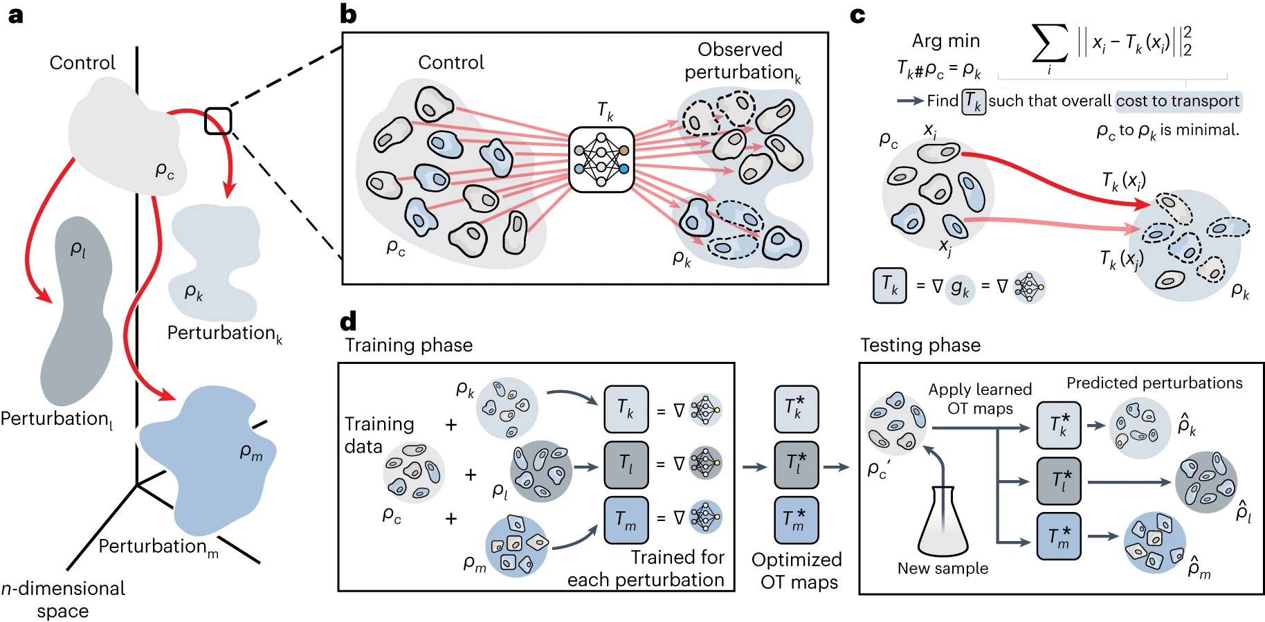
上图是它的研究方法。

CellOT outperforms state-of-the-art methods

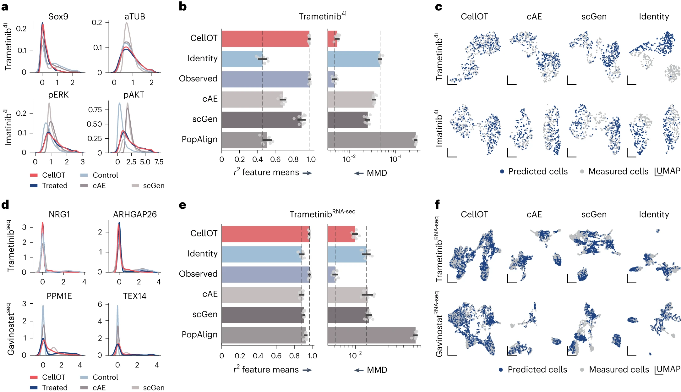
这里的图a和d主要是看CellOT的线和Treated的线的重合程度。而且这里越重合越能说明CellOT更好的把握到了里面细微的结构。

CellOT captures cell-to-cell variability in drug responses

这里的图b旨在说明pERK(phosphorylation levels of extracellular signal-regulated kinases)水平，预测和真实值的分布相似，这是由于信号激酶的水平和治疗后的细胞状态是紧密相关的。

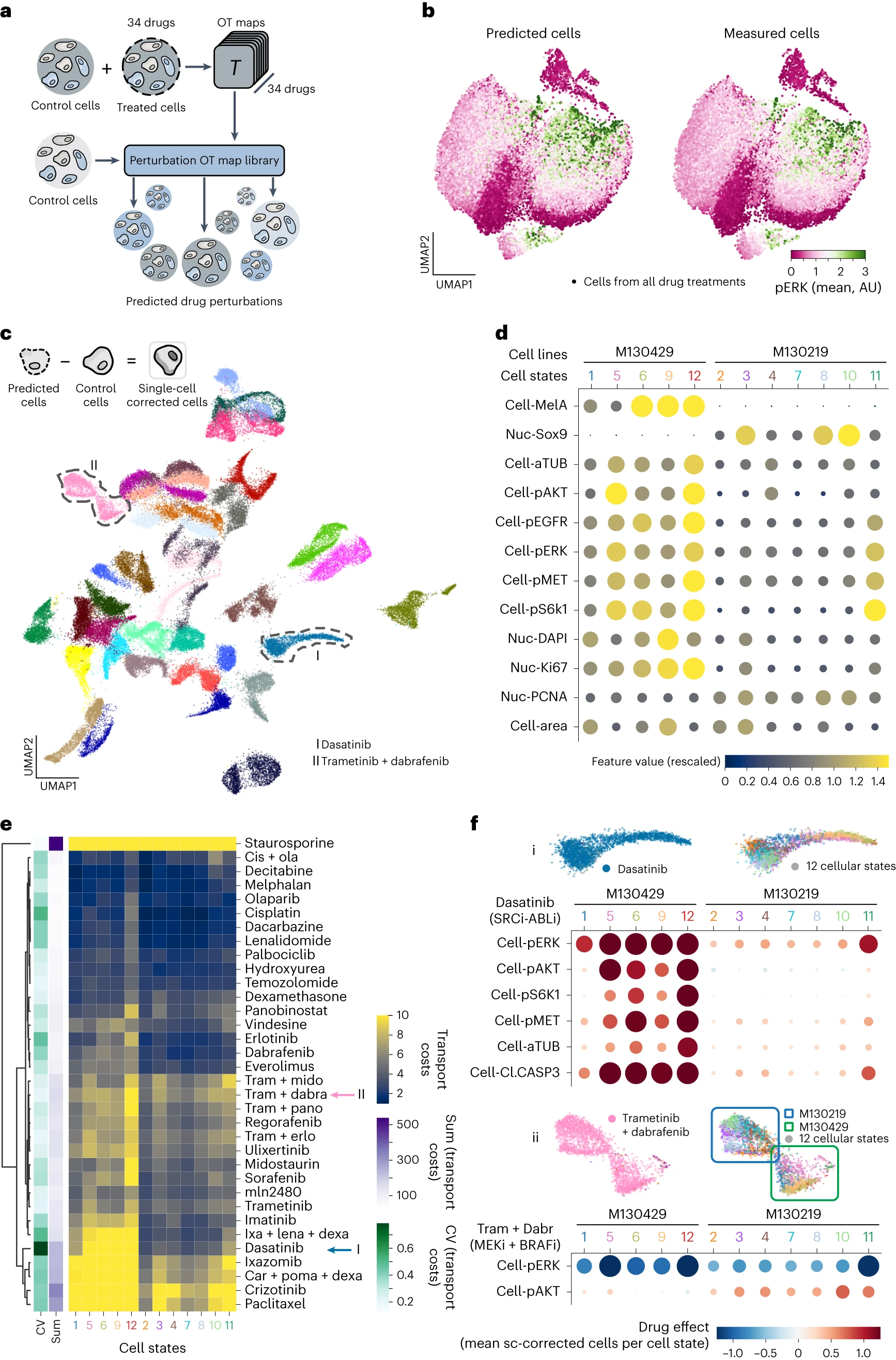
CellOT disentangles subpopulation-specific drug effects

上面的图c表示，CellOT可以通过计算预测细胞和control细胞的差分来分离每种药物的作用模式。

（这里并不是很清楚它的实现方法，后面看看代码）

上面的图d有点类似于细胞注释的方法，先对其进行聚类，然后根据聚类和基因的结果来对类进行注释。

Computing the difference between the control and treated state of each drug (the optimal transport cost), allows us to further characterize a drug’s severity.这里的意思是，如果transport cost越大，说明经过细胞扰动后的细胞的变异程度越大，像是Staurosporine是细胞凋亡剂基本上Transport cost拉满了。

图f说明了dasatinib特异性的诱导了5，6，9，19的死亡。

CellOT accurately infers cellular responses in unseen patients

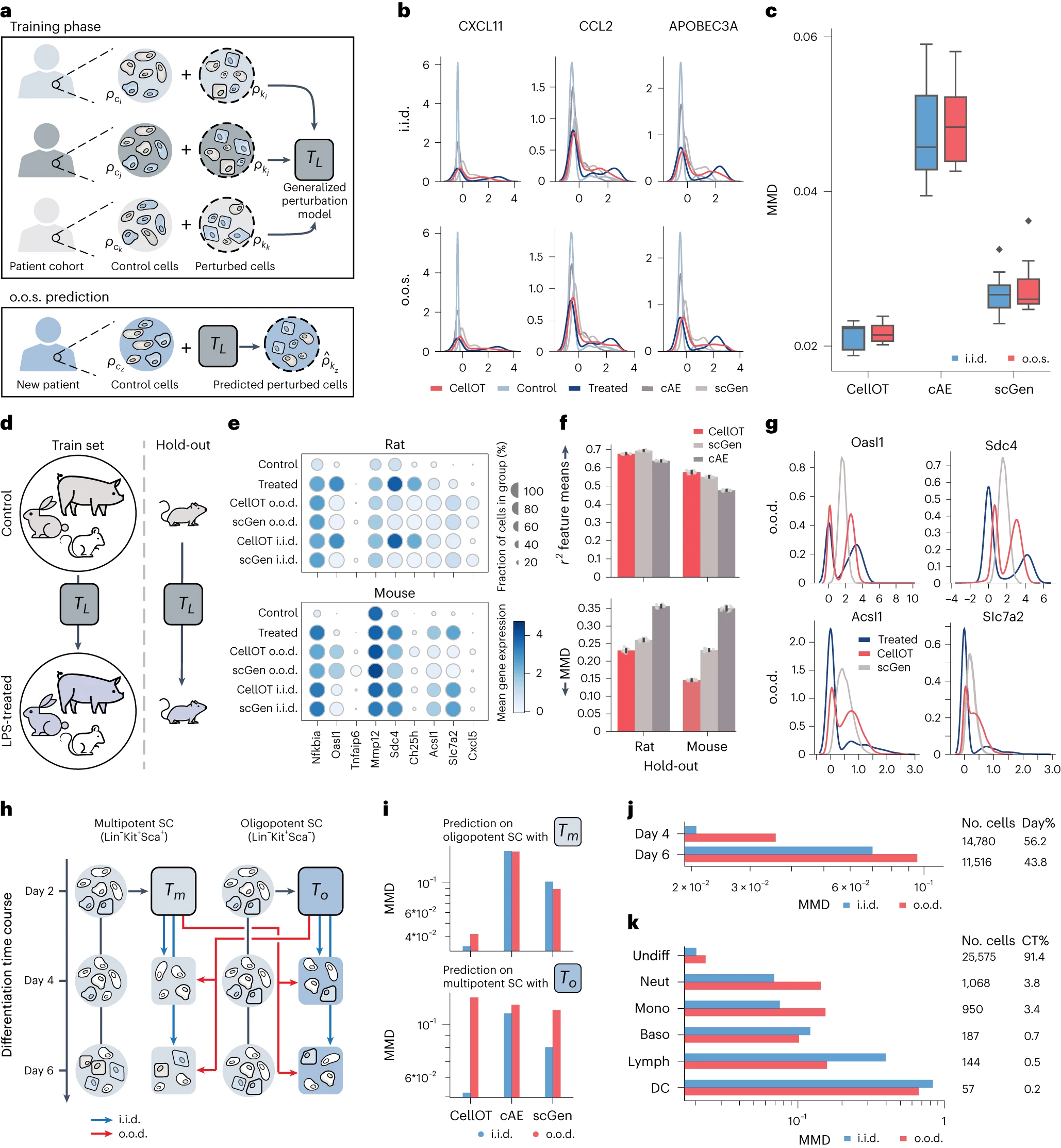
这里的i.i.d.指的是独立同分布，即模型能够看到所有患者的细胞。o.o.s.指的是样本外设定，即模型在训练时看不到特定保留患者的细胞。更通俗来说是新来了一个患者，我们不知道它的细胞就直接对他进行预测。

可以看到，在从i.i.d.推广到o.o.s.时性能下降较小。但如果队列规模较小且每个个体的响应存在高度差异，你们泛化能力会受到挑战。

CellOT reconstructs innate immune responses across species

上图d：We refer to the generalization task as out-of-distribution (o.o.d.), as unlike the o.o.s. setting, we expect different species to have very distinct responses

图f能一定程度反应CellOT好在哪，但g图更直观的反映了CellOT可以把握里面更细微的结构。

这里也能看出同样的细胞在不同的物种之间的差异也是很大的，环境对细胞的影响也不容忽视。

CellOT extends differentiation results to cells of lower potency

By tracking an initial cell population along the differentiation process, CellOT allows us to recover individual molecular cell-fate decisions and developmental trajectories.

$T_o$针对寡能细胞进行训练，而$T_m$针对多能细胞进行训练。

这里也很好理解为什么$T_o$对于multipotent的训练不太行，从单调的到复杂的肯定泛化能力不行。

Methods

补充

MMD

Maximum Mean Discrepancy (MMD)。

1. 基本概念

MMD，全称 Maximum Mean Discrepancy，是一种用来衡量两个分布之间差异的统计量。
它的核心思想是：

如果两个分布相同，那么在某个合适的函数空间中，它们的“均值嵌入”应该相等。
反之，如果嵌入不相等，就说明分布不同。

它广泛用于 分布对齐、域自适应、生成模型评估 等场景，比如比较生成模型产生的数据和真实数据的分布差异。

2. 数学定义

设有两个分布：

$P$ （比如真实数据分布）
$Q$ （比如生成数据分布）

我们从它们中各取样本：

$$\begin{equation}
X = {x_1, x_2, \dots, x_m} \sim P, \quad Y = {y_1, y_2, \dots, y_n} \sim Q
\end{equation}$$

MMD 定义为：

$$\begin{equation}
\text{MMD}[\mathcal{F}, P, Q] = \sup_{f \in \mathcal{F}} \left( \mathbb{E}{x \sim P}[f(x)] - \mathbb{E}{y \sim Q}[f(y)] \right)
\end{equation}$$

其中：

$\mathcal{F}$ 是一个函数类（通常取再生核希尔伯特空间 RKHS 里的函数集合）。
直观理解：找到一个“最能区分”两个分布的函数 $f$，用它来放大两者的差异。

3. 核方法形式

如果选择 $\mathcal{F}$ 为 RKHS 对应的单位球函数空间，MMD 有一个非常漂亮的核函数形式：

$$\begin{equation}
\text{MMD}^2(P, Q) = \mathbb{E}{x,x’ \sim P}[k(x,x’)] + \mathbb{E}{y,y’ \sim Q}[k(y,y’)] - 2\mathbb{E}_{x \sim P, y \sim Q}[k(x,y)]
\end{equation}$$

其中 $k(\cdot, \cdot)$ 是核函数（常用 RBF 高斯核）。

样本估计（无偏估计）：

给定样本 ${x_i}{i=1}^m, {y_j}{j=1}^n$，估计式是：

$$\begin{equation}
\text{MMD}^2 = \frac{1}{m(m-1)} \sum_{i \neq i’} k(x_i, x_{i’})

\frac{1}{n(n-1)} \sum_{j \neq j’} k(y_j, y_{j’})

\frac{2}{mn} \sum_{i,j} k(x_i, y_j)
\end{equation}$$

4. 直观理解

如果 $P=Q$，那么 MMD → 0。
如果 $P \neq Q$，MMD 会大于 0。
MMD 越大，说明两个分布差异越大。

相比于 KL 散度、JS 散度 等方法，MMD 的优势是：

不需要估计分布的密度，直接基于样本就能计算。
在高维数据（如图像）上更实用。

5. 应用场景

生成对抗网络 (GAN) 评估：MMD 用于衡量生成数据和真实数据分布的差异。
域自适应 (Domain Adaptation)：MMD 常作为 loss，来让源域和目标域的特征分布更接近。
假设检验 (Two-sample test)：判断两个样本集合是否来自同一分布。