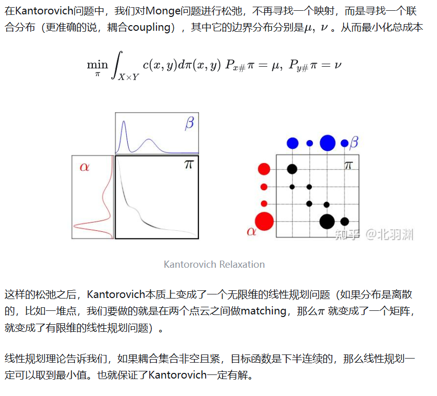
1
2
3
4
5
6
7
8
9
10
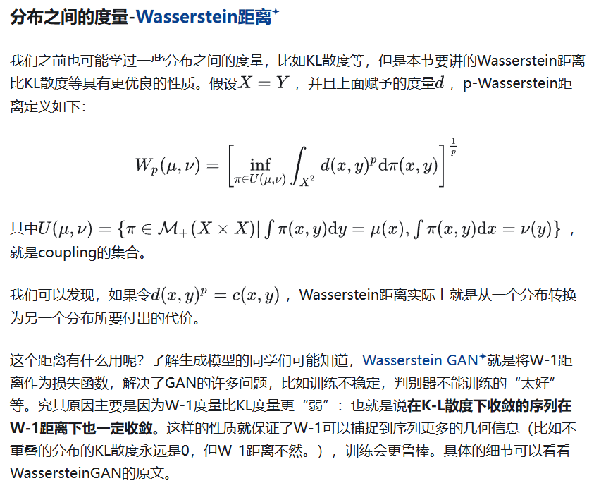
11
12
13
14
15
16
17
18
19
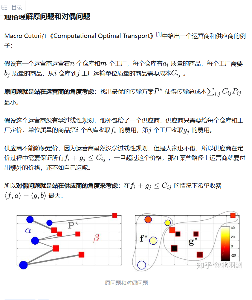
20
21
22
23
24
25
26
27
28
29
30
31
32
33
34
35
36
37
38
39
40
41
42
43
44
45
46
47
48
49
50
51
52
53
54
55
56
57
58
59
60
61
62
63
64
65
66
67
68
69
70
71
72
73
74
75
76
77
78
79
80
81
82
83
84
85
86
87
88
89
90
91
92
93
94
95
96
97
98
99
100
101
102
103
104
105
106
107
108
109
110
111
112
113
114
115
116
117
118
119
120
121
122
123
124
125
126
127
128
129
130
131
132
133
134
135
136
137
138
139
140
141
142
143
144
145
146
147
148
149
150
151
152
153
154
155
156
157
158
159
160
161
162
163
164
165
166
167
168
169
170
171
172
173
174
175
176
177
178
179
180
181
182
183
184
185
186
187
188
189
190
191
192
193
194
195
196
197
198
199
200
201
202
203
204
205
206
207
208
209
210
211
| ### 第三个,怎么利用拉格朗日对偶形式
#### 2. 拉格朗日对偶思路 (Lagrangian Duality)
为什么会出现对偶形式(带 $g(x)+f(y) \le c(x,y)$ 的公式)呢?这是 **拉格朗日对偶**的典型应用。思路分几步:
---
###### (1) 原始问题 (Primal)
写成积分形式:
$$
\min_{\gamma \ge 0} \int c(x,y)\, d\gamma(x,y)
$$
约束:
$$
\int d\gamma(x,y) = \mu(x), \quad \int d\gamma(x,y) = \nu(y).
$$
也就是说:
* $\gamma$ 的 $x$-边际是 $\mu$;
* $\gamma$ 的 $y$-边际是 $\nu$。
---
###### (2) 给约束加拉格朗日乘子
用函数 $g(x)$、$f(y)$ 作为拉格朗日乘子,写成拉格朗日函数:
$$
L(\gamma, g,f) = \int c(x,y)\, d\gamma(x,y)
+ \int g(x)\, \big( d\mu(x) - \int d\gamma(x,y)\big)
+ \int f(y)\, \big( d\nu(y) - \int d\gamma(x,y)\big).
$$
展开后得到:
$$
L(\gamma,g,f) = \int g(x)\, d\mu(x) + \int f(y)\, d\nu(y) + \int \big(c(x,y) - g(x) - f(y)\big)\, d\gamma(x,y).
$$
---
###### (3) 取 inf over $\gamma$
* 我们希望 $\min_\gamma L(\gamma,g,f)$ 是良定义的。
* 如果 $c(x,y) - g(x) - f(y) < 0$ 在某处成立,那么对那个地方的 $\gamma(x,y)$ 可以趋向无穷大,就会让 $L$ 趋向 $-\infty$。
* 为了避免这种情况,必须要求
$$
g(x) + f(y) \le c(x,y), \quad \forall (x,y).
$$
这就是你看到的条件。
于是 $\inf_\gamma L(\gamma,g,f) = \int g\, d\mu + \int f\, d\nu$,如果满足约束,否则是 $-\infty$。
---
###### (4) 得到对偶问题 (Dual)
所以对偶问题就是:
$$
\sup_{g,f} \;\; \int g(x)\, d\mu(x) + \int f(y)\, d\nu(y) \quad
\text{s.t.}\quad g(x)+f(y)\le c(x,y).
$$
这就是 **Kantorovich 对偶形式**。
## Villani对于这个dual问题的转化
$$\begin{equation}
W(\mu, \nu)= \underbrace{\frac{1}{2}{\mathbb{E}}\left[\|x\|_{2}^{2}+\|y\|_{2}^{2}\right]}_{{\mathcal{C}}_{\mu, \nu}}-\min _{f \in {\tilde{\mathrm{\Phi}}}} {\mathbb{E}}_{\mu}[f^{*}(x)]+{\mathbb{E}}_{\nu}\left[f(y)\right],
\end{equation}$$
where
$\widetilde{{{\Phi }}}$ is the set of all convex functions in $L1(dμ) × L1(dν)$, L1(μ):={g is measurable & ∫gdμ < ∞} , ${f}^{* }(x)=\mathop{\max }\nolimits_{y}\langle y,x\rangle -f(y)$ is f’s convex conjugate, and the optimal transport map transforming μ into ν corresponds to the gradient of $f*$, i.e., $T = ∇ f*$. We can recover the optimal transport plan via $\gamma ={(\nabla {f}^{* }\times {{{\rm{Id}}}})}_{\sharp }\mu$
. Theorem 2.9 by Villani23 then proves the existence of an optimal pair $(f, f*)$ of lower semi-continuous proper conjugate convex functions on $\mathbb{R}^n$
minimizing (3).
这一大段我就看不懂了,我也不想看懂了。
但还是顺便理解一下凸共轭
### 凸共轭
好问题 👍。**凸共轭 (convex conjugate)** 是凸分析里的一个核心概念,直觉上它描述了一个函数在所有可能“斜率”下的“最佳线性近似”。我帮你拆开:
---
1.定义
给定一个函数 $f:\mathbb{R}^d \to \mathbb{R}\cup\{+\infty\}$,它的 **凸共轭** $f^*$ 定义为:
$$
f^*(x) = \sup_{y \in \mathbb{R}^d} \{\langle x, y \rangle - f(y)\}.
$$
* $\langle x, y\rangle$ 是一个线性函数(斜率由 $x$ 决定)。
* $\langle x, y\rangle - f(y)$ 表示“线性函数 $\langle x, y\rangle$”减去原函数的值。
* 对所有 $y$ 取最大值,得到的就是 $f^*(x)$。
👉 换句话说:
**$f^*(x)$ 衡量的是:斜率为 $x$ 的线性函数,能在多大程度上“支撑”或“逼近”原函数 $f$。**
因此,凸共轭可以理解为 **“函数的斜率空间里的重新表达”**。
* 如果 $f(y)$ 是一个凸函数,那么在平面上可以画很多条直线(仿射函数):
$$
\ell_x(y) = \langle x, y\rangle - b
$$
想要让直线 $\ell_x$ 永远在 $f(y)$ 下面,$b$ 必须足够大。
* 那么 $f^*(x)$ 正是这个最小 $b$ 的负数,也就是“用斜率 $x$ 的直线支撑函数 $f$ 的代价”。
所以 **共轭操作就是把函数换一种坐标:从“点空间 (y)”切换到“斜率空间 (x)”**。
例1:二次函数
$$
f(y) = \tfrac12\|y\|^2.
$$
计算共轭:
$$
f^*(x) = \sup_y \{\langle x,y\rangle - \tfrac12\|y\|^2\}.
$$
最大值出现在 $y=x$,所以:
$$
f^*(x) = \tfrac12\|x\|^2.
$$
➡️ 二次函数的共轭还是自己。
---
例2:指示函数
若
$$
f(y) = \begin{cases}
0 & y\in C, \\
+\infty & y \notin C,
\end{cases}
$$
则
$$
f^*(x) = \sup_{y\in C} \langle x,y\rangle,
$$
这就是集合 $C$ 的 **支撑函数**。
---
* **双共轭**:$f^{**}=f$ (若 $f$ 是凸的、下半连续)。这叫 **Fenchel-Moreau 定理**。
* 共轭把“点值视角”转为“斜率视角”,特别适合与最优传输里的**梯度映射**搭配。
* 在 OT 里,最优传输映射 $T=\nabla f^*$,正是利用了“凸函数的梯度”能编码一个单值映射的性质。
**总结**:
凸共轭 $f^*$ 就是把函数 $f$ 从“点空间”转到“斜率空间”的表达,它告诉我们用斜率为 $x$ 的线性函数去支撑 $f$ 的最优程度。它在几何上对应支撑函数,在优化与 OT 里是把函数与映射(梯度)联系起来的桥梁。
##
$$\begin{equation}
W(\rho_c, \rho_k)=\max\limits_{\substack{f \in {\tilde{\mathrm{\Phi}}} \\ f^{*} \in L^{1}(\rho_k)}} \min\limits_{g \in {\tilde{\mathrm{\Phi}}}} {\mathcal{C}}_{\rho_c, \rho_k} \underbrace{-{\mathbb{E}}_{\rho_c}[\langle x, \nabla g(x)\rangle-f(\nabla g(x))] - {\mathbb{E}}_{\rho_k}[f(y)]}_{{\mathcal{V}}_{\rho_c, \rho_k}(g, f)}.
\end{equation}$$
好的,我来逐句帮你翻译并解释这段话:
---
$$
W(\mu, \nu)= \underbrace{\frac{1}{2}{\mathbb{E}}\left[\|x\|_{2}^{2}+\|y\|_{2}^{2}\right]}_{{\mathcal{C}}_{\mu, \nu}}-\min _{f \in {\tilde{\mathrm{\Phi}}}} {\mathbb{E}}_{\mu}[f^{*}(x)]+{\mathbb{E}}_{\nu}\left[f(y)\right],
$$
其中:
* **$\widetilde{\Phi}$** 表示所有凸函数的集合,这些函数属于 $L^1(d\mu) \times L^1(d\nu)$。
* $L^1(\mu):={g \ \text{是可测函数 且} \int g , d\mu < \infty }$,即在测度 $\mu$ 下可积的函数集合。
* **$f^*(x)=\max_y \langle y, x \rangle - f(y)$** 是函数 $f$ 的 **凸共轭(convex conjugate)**。
* 将 $\mu$ 转换为 $\nu$ 的最优传输映射(optimal transport map)对应于 $f^*$ 的梯度,即
$$
T = \nabla f^*.
$$
* 我们可以恢复最优传输计划(transport plan):
$$
\gamma = (\nabla f^* \times \mathrm{Id})_\sharp \mu,
$$
其中 $(\cdot)\_\sharp \mu$ 表示 **推前测度(pushforward measure)**。
* Villani 的《最优传输理论》(Theorem 2.9)证明了:在 $\mathbb{R}^n$ 上,存在一对最优的 $(f, f^*)$,它们是下半连续(lower semi-continuous)、适当的(proper)且互为凸共轭函数,并且它们能够最小化上式中的优化问题 (3)。
|