# Title

Systema: a framework for evaluating genetic perturbation response prediction beyond systematic variation

# Abstract

# 什么是系统变异

Systematic variation：the consistent transcriptional differences between perturbed and control cells arising from selection biases or confounders.

# Metrics

common metrics are susceptible to these biases, leading to overestimated performance.

# 文章的结论

Using this framework, we uncover insights into the predictive capabilities of existing methods and show that predicting responses to unseen perturbations is substantially harder than standard metrics suggest. Our work highlights the importance of heterogeneous gene panels and disentangles predictive performance from systematic effects, enabling biologically meaningful developments in perturbation response modeling.

# Main

# Background

Recent advances in high-throughput perturbation screening technologies have enabled unprecedented opportunities to systematically investigate the effects of perturbations in diverse cellular contexts; however, the space of possible perturbations is combinatorially complex, making exhaustive experimental exploration infeasible.

对于模型而言，已经有许多模型用复杂的深度学习框架去学习扰动后的基因表达，但是表现不如简单的模型。

引出问题：to what extent are existing perturbation response prediction methods learning the perturbation biology of single cells?

现有的扰动预测模型在多大程度上学习了单细胞中扰动的生物信息

# 模型实现：

We introduce a measure to quantify the degree of systematic variation in perturbation datasets, and we posit that existing metrics are susceptible to these systematic biases, which can often lead to misleading conclusions.

Systema：

• mitigates systematic biases by focusing on perturbation-specific effects
• provides an interpretable readout of the methods’ ability to reconstruct the perturbation landscape.

# Results

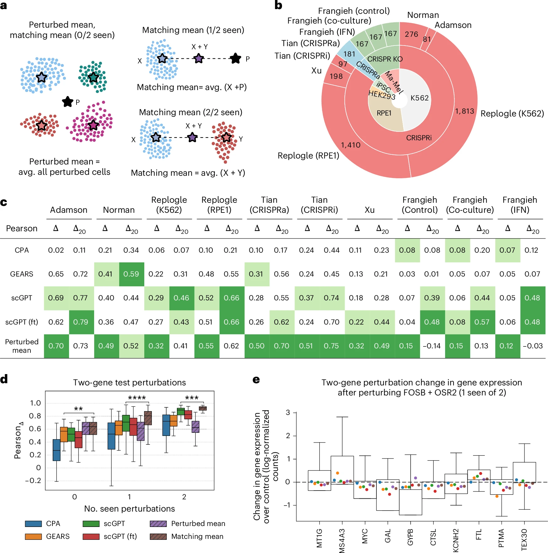
这篇文章设计了两种简单的 nonparametric baselines，如图 a 所示。下面给出它的计算公式

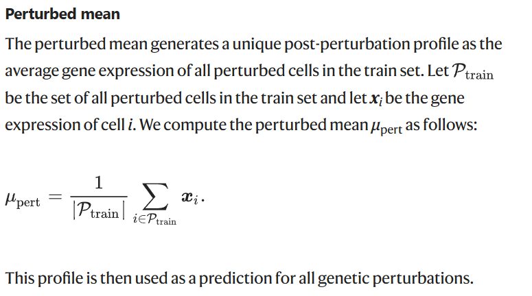
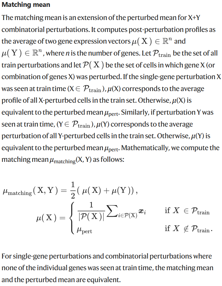
图 c 是皮尔逊相关系数去衡量 how well different methods can predict the transcriptional changes of a perturbation with respect to the population of control cells. 进而去回答前面提到的问题。这里需要注意的是图 c 是 unseen one-gene perturbation

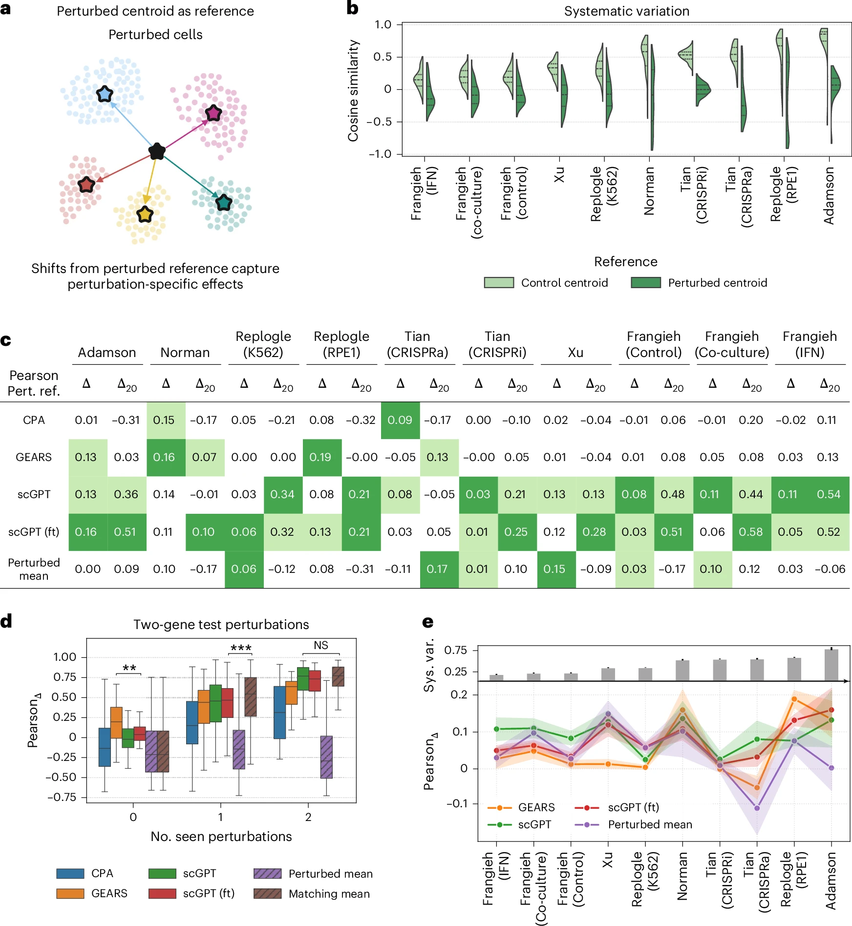
图 d 是 Norman dataset，使用的是 two-gene perturbations in the Norman dataset.

图 e 表示大部分扰动响应模型主要是捕捉到了系统的偏差而没有捕捉到 perturbation-specific effects.

# Systematic differences between control and perturbed cells lead to high predictive scores

systematic variation can lead to overestimated predictive performance of perturbation response models when they primarily capture the average perturbation effect, obscuring their ability to generalize to novel perturbations.

In perturbation datasets, systematic differences between perturbed and control cells may be explained by potential selection biases, confounding variables or underlying biological factors.

下面一大段举了一下为什么有 systematic，例子看着挺新鲜的：perturbing a panel of functionally related genes will lead to transcriptomic profiles that are consistently different between perturbed and control cells.

Additionally, unmeasured variables such as cell-cycle phase, chromatin landscape and target efficiency may strongly influence post-perturbation profiles21. 即使是相同的扰动，不同细胞由于处于不同的 “背景状态”，结果也可能不同。

Systematic variation may still arise when responses that are biological in origin but systematic in effect, such as stress response or cell-cycle arrest, occur broadly across many perturbations. 这些效应虽然不是 “噪声”，但它们会掩盖或混淆扰动本身的特异性效应。

这里做实验使用了两个数据集，第一个是 Adamson 数据集，主要针对内质网稳态的相关基因进行扰动（预计会在内质网功能相关的通路上表现出差异）

第二个是 Norman 数据集，主要针对细胞周期和细胞生长相关基因进行扰动，预计细胞会在细胞周期、增殖相关的通路上表现出差异。

通过 GESA (gene set enrichment analysis) 检测哪些基因在扰动细胞内被显著激活或抑制。（GESA 不看单个基因，而是看一组具有共同功能通路的基因整体在条件之间是否表现出富集的趋势。

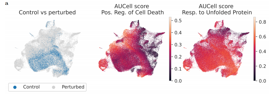
同时也利用 AUCell 去衡量每个单细胞的活动。

AUCell 的方法：

1. 对每个细胞的基因表达值做排序（高表达的基因排在前面）。
2. 看目标基因集的基因在这个排序里处于什么位置。
3. 计算一个 AUC (Area Under the Curve, 曲线下面积) 值，反映这些基因是否集中出现在前面（高表达区域）。
   

这个图里面有很多东西可以去学习：

---

# 1. enrichment score (ES)

在 GSEA（基因集富集分析） 里，enrichment score 表示：

某个基因集（比如一个通路）在差异基因排序列表里 “靠前 / 靠后” 的程度。

• 越靠前 → 说明这个基因集整体上 上调。
• 越靠后 → 说明这个基因集整体上 下调。

---

# 2. normalized enrichment score (NES)

问题：不同基因集大小不同（有的基因集只有 20 个基因，有的可能有 200 个）。

• 如果直接比较 ES，大的基因集天然更容易得到极端值。
• 解决方法：对 ES 做归一化 → 得到 NES。

👉 NES 就是一个可以直接比较的指标，反映该基因集相对于背景的富集强度。

---

# 3. false discovery rate (FDR, 假发现率)

• 因为我们在分析很多基因集（可能几百上千），要考虑 多重检验校正。
• FDR 就是多重比较校正后的显著性指标，告诉你 “这个通路的富集结果有多少可能是假的”。
• 通常 FDR < 0.05 就认为是显著的。

---

# 4. top enriched pathways

指的是 富集程度最高、最显著的通路。

• 例如细胞周期、DNA repair、免疫应答等。
• “top” 就是按照 NES 或 FDR 排序，选出来的最有意义的一批通路。

📌 类比一下：
就好比你做了一场考试（差异表达分析），然后统计某些 “学生群体”（基因集）是否整体分数特别高（上调）或特别低（下调）。

• NES = 这个群体的成绩偏高 / 偏低的程度。
• FDR = 这个群体成绩 “真的很不一样” 的置信度。
• top enriched pathways = 表现最极端的一些群体。

这张图表现出来他们的 FDR 都很低，说明这个结果的可信度比较高。

上面这个图不知道怎么看的

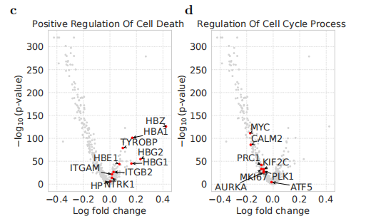
这图里面标注的基因都是对应调节的基因，例如对于 Cell Death 它的基因都倾向于明显被上调，也就是处于 V 字火山图的右侧，而 Cell cycle 的基因大多被下调

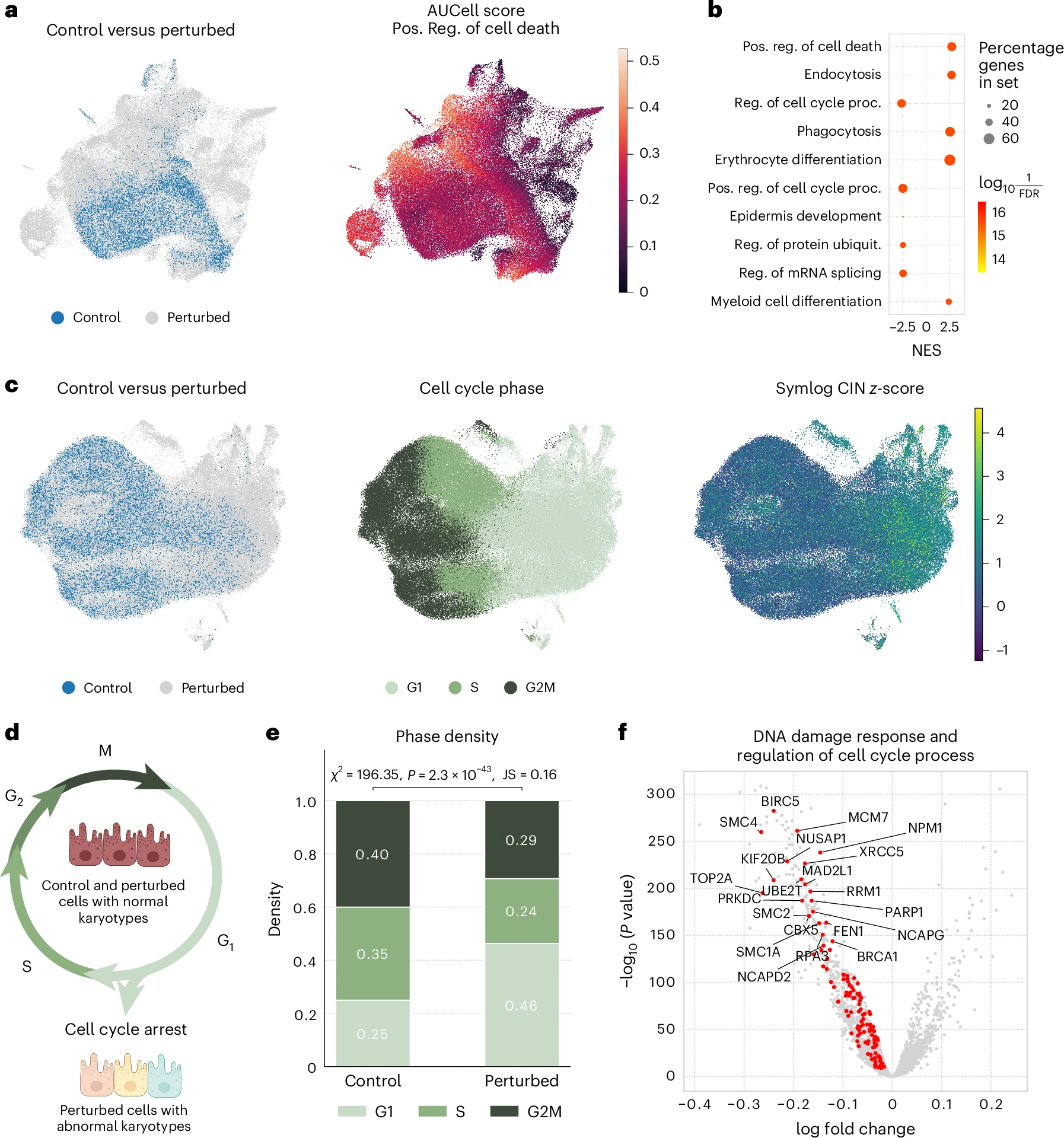
c-e 图展示了在 Replogle data-set 上做的实验。

这给出了为什么他认为在 G1 阶段的 perturbed 细胞多于 control 细胞：We attribute this effect to the widespread chromosomal instability induced by perturbations; p53-positive RPE1 cells with abnormal karyotypes tend to react to instabilities through cell-cycle arrest

后面会附上对于 Jensen-Shannon divergence 的解释

这里他也做了对比的一个实验：

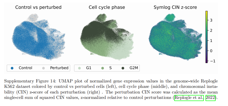
对于上图的 K562 数据集，由于它的 p53 呈阴性，所以在细胞循环的差异就没有那么大。

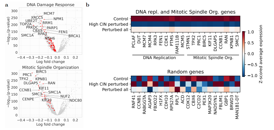
Genes belonging to the enriched RPE1 pathways had consistently lower expression in perturbed cells than in control cells, reflecting the high prevalence of chromosomal instabilities among perturbed cells

# Standard reference-based metrics are susceptible to systematic variation

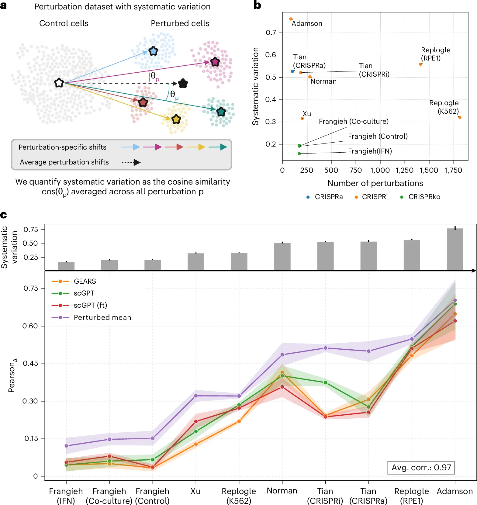
图 a：To quantify systematic variation, we computed the distribution of cosine similarities between perturbation-specific shifts and the average perturbation effect

图 b： the degree of systematic variation differed considerably among the ten datasets considered in our benchmark

图 c：systematic variation 的高低影响了皮尔逊系数的高低。

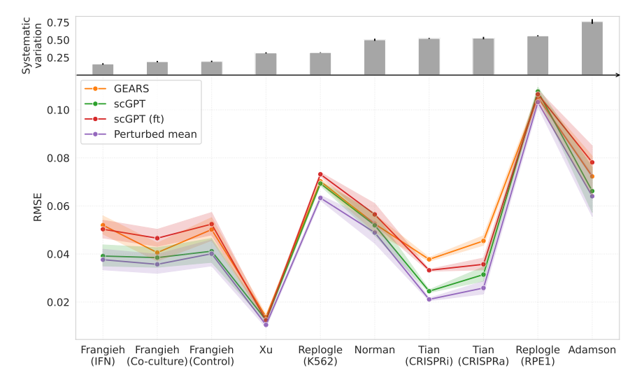
RMSE 收到的影响更少，mean-squared error 也更少。

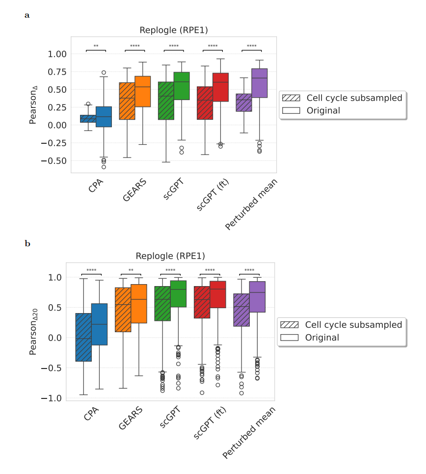
这里把 perturbation 的数据降采样为和 control cell 一样的 phase distribution 然后对各个模型进行比较。

# Evaluating the prediction of perturbation-specific effects

# 附

# Jensen–Shannon divergence (JSD, Jensen–Shannon 散度)

是信息论里常用的一个 衡量两个概率分布差异的指标。我帮你分层解释一下：

---

# 1. 背景

• 在统计和机器学习里，我们经常要比较 两个概率分布 P 和 Q 是否相似。
• 最常见的指标是 KL 散度 (Kullback–Leibler divergence)：

\begin{equation} KL(P||Q) = \sum_x P(x)\,\log\frac{P(x)}{Q(x)} \end{equation}

但是 KL 有两个问题：

• 不对称（KL (P||Q) ≠ KL (Q||P)）
• 如果 Q (x)=0 而 P (x)≠0，就会发散成 ∞

---

# 2. Jensen–Shannon 散度的定义

为了解决 KL 的缺陷，JSD 出现了。

定义：

\begin{equation} JSD(P||Q) = \frac{1}{2} KL(P||M) + \frac{1}{2} KL(Q||M) \end{equation}

其中

\begin{equation} M = \frac{1}{2}(P+Q) \end{equation}

是 P 和 Q 的平均分布。

---

# 3. 特点

• 对称性：JSD (P||Q) = JSD (Q||P)

• 有界性：取值范围在 [0, 1]（如果用 log base 2）。

  • JSD = 0 → 两个分布完全相同
  • JSD 越大 → 两个分布差异越大，最大值 = 1

• 平滑性：不会像 KL 那样出现无穷大，因为它用平均分布 M 缓和了差异。

---

# 4. 举个例子

假设我们有两个分布：

• P = (0.9, 0.1)

• Q = (0.1, 0.9)

• KL (P||Q) 很大（因为差异太大）

• JSD (P||Q) ≈ 0.76（log base 2），说明分布差异大，但有限制在 0~1 之间。

---

# 5. 应用

• 自然语言处理：比较两个文本的词频分布差异
• 生物信息学：比较细胞群体的基因表达分布差异
• 聚类与分类：衡量不同类之间的分布差异

---

✅ 一句话总结：
JSD 是一个对称、有限的分布差异度量，常用来比较两个概率分布的相似性，比 KL 散度更稳定。