SpaGCN: Integrating gene expression, spatial location and histology to identify spatial domains and spatially variable genes by graph convolutional network.

主要利用了 spage2vec 方法对数据进行降维便于聚类，在拟合神经网络的时候利用 DEC 方法作为 loss 函数，创造了一种分辨 SVG 基因（提取 meta-gene）的方法。

生词基本上都记住了，这次就直接从文章入手吧。

# 摘要

Through graph convolution, SpaGCN aggregates gene expression of each spot from its neighboring spots, which enables the identification of spatial domains with coherent expression and histology.

we show it can detect genes with much more enriched spatial expression patterns than competing methods.

# Introduction

methods for SRT:

in situ hybridization or sequencing-based technologies with single-cell resolution
- e.g. seqFISH, seqFISH+, MERFISH, STARmap and FISSEQ that measure the expression level for hundred to thousands of genes in cells within their tissue context.
- 因为能达到单细胞分辨率，这些技术适合于高精度分析，用于深入理解细胞在组织结构中的分布以及细胞间的相互作用。
in situ capturing-based technologies with spatial barcoding followed by sequencing
- e.g. spatial transcriptomics(ST), SLIDE-seq, SLIDE-seqV2, HDST and 10x Visium that measure the expression level for thousands of genes in captured locations, referred to as spots.
- 由于通常只能定位到捕获区域的水平，这类技术的空间分辨率低于单细胞分辨率，但它们适合于大规模研究，因为能够同时检测数千个基因。

identifying spatial domains account for spatial dependency ---- spatial dependency of gene expression:
- Hidden-Markov random field(HMRF)
- stLearn
- BayesSpace
flaws: the lack of flexibility with different modalities has made the less versatile.
最直观的 SpaGCN 适用于 imaging-based 的数据，这几个不行。然而可以从 Benchmark 那篇文章看出来，这个 SpaGCN 对于 Multi-splice 的数据也是没辙。
Detect spatially variable genes(SVGs): Trendscreek, SpatialDE and SPARK.
- These methods examine each gene independently and return a P value to represent the spatial variability of a gene.
- due to the lack of consideration of spatial domains, genes detected by these methods do not have guaranteed spatial expression patterns.

SpaGCN 同时考虑上述两种问题：

SpaGCN first identifies spatial domains by integrating gene expression, spatial location and histology through the construction of an undirected weighted graph that represents the spatial dependency of the data.
For each spatial domain, SpaGCN then detects SVGs that are enriched in the domain.
By restricting the search space to spatial domains, the SVGs detected by SpaGCN are guaranteed to have spatial expression patterns.

# Result

# Overview of SpaGCN and evaluation

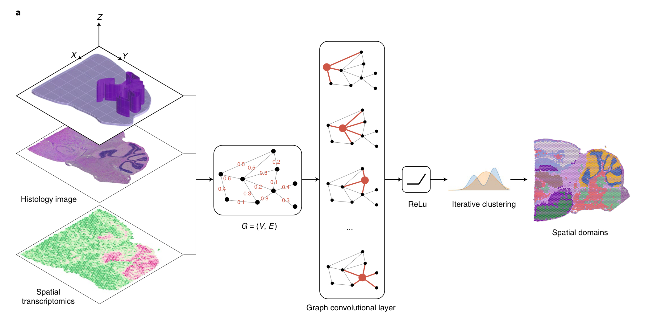
SpaGCN first builds a graph to represent the relationship of all spots considering both spatial location and histology information.
SpaGCN utilizes a graph convolutional layer to aggregate gene expression information from neighboring spots.
SpaGCN uses the aggregated expression matrix to cluster spots using an unsupervised iterative clustring algorithm.

Each cluster is considered as a spatial domain from which SpaGCN then detects SVGs that are enriched in a domian by DE analysis.

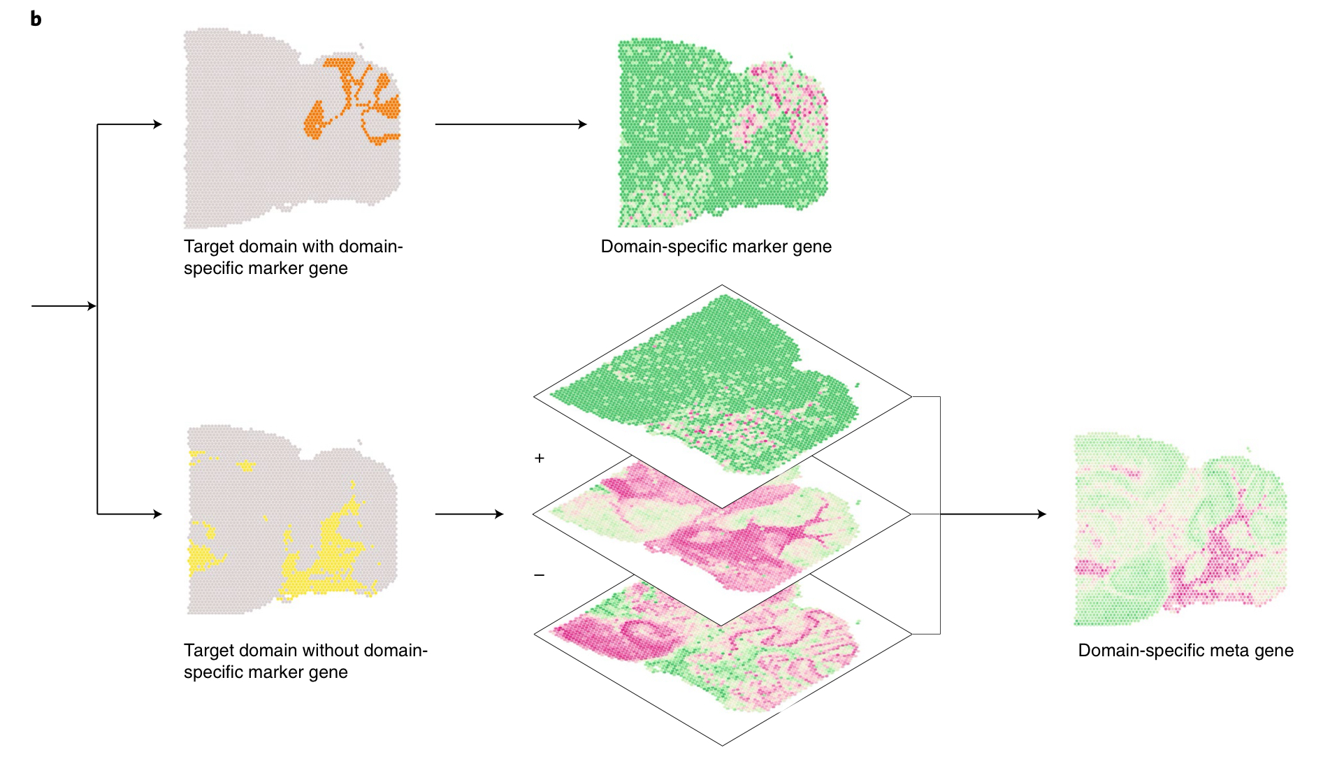
When a single gene cannot mark the expression pattern of a domain, SpaGCN will construct a meta gene, formed by the combination of multiple genes, to represent the expression pattern of the domain.

# Application to human primary pancreatic (胰腺的) cancer ST data

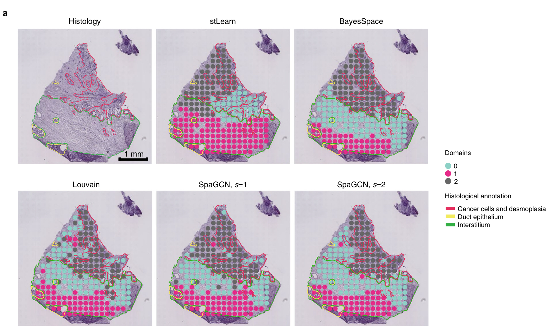
这张图利用各种算法对于 cancer region 的检测，相当于对比一下之前提到的第一个，分类任务
desmolasia: 结缔组织增生
Duct epithelium: 导管上皮
interstitium: 间质

说实话，我没看懂这图中 SpaGCN 比 Louvain 好在哪了，但是灵活性在 s 这个参数倒是体现的很好

parameter s, which controls the weight given to histology when detecting neighbors for each spot.

接下来是检测 SVGs.
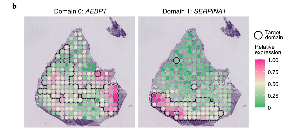
这张图代表了 Spatial expression pattern of SVGs detected by SpaGCN for domain 0 (AEBP1) and domain 1 (SERPINA1)

我最开始误以为这图里面就对应着有 3，8 个 SVGs，然而这个图代表的是其中某一个 SVG 的表征。SVG 的意思是 Spatially Variable genes，当它在不同的区域的基因表现是一样的时候，那么它就不是 SVG，如果它在不同的区域，基因的表现存在高表达，那么它就是 SVG。

In total, SpaGCN detected 12SVGs, with three, eight and one SVGs for domain0 , 1, 2, respectively

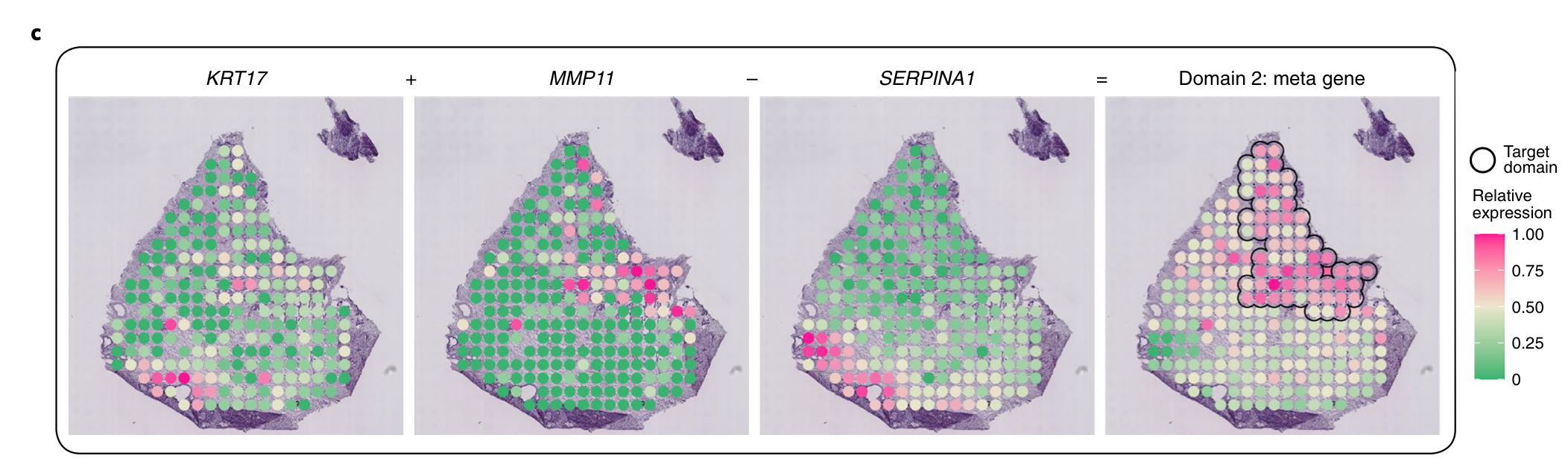
Spatial expression patterns of genes KRT17, MMP11, SERPINA1, which form the meta gene for domain 2 (KRT17+MMP11-SERPINA1).

KRT17 functions as a tumor promoter and regulates proliferation in pancreatic cancer, and MMP11 is a prognostic biomarker for pancreatic cancer.

SPARK and SpatialDE 检测出来 203 和 163 个 SVGs，但是他们的 P 或 Q values 偏斜 (skew) 到了 0.
在统计学和生物信息学中，p 值（p-value） 和 q 值（q-value） 是用来衡量数据显著性的指标：
# 1. P 值（p-value）
定义：p 值表示在假设原假设为真的情况下，观测到的数据或更极端数据的概率。
解释：p 值用于检验数据是否具有统计显著性。一个较低的 p 值（例如小于 0.05）表明在原假设成立的情况下，观测到的结果极不可能，因此通常拒绝原假设。
用途：常用于单次假设检验，帮助判断结果是否具有统计显著性。
局限性：在多重假设检验（同时进行多个检验）中，单纯使用 p 值容易产生多重比较问题，即假阳性结果（false positives）增加。
# 2. Q 值（q-value）
定义：q 值是多重检验中的一个校正后的 p 值，代表的是 “错误发现率”（ False Discovery Rate, FDR） 。FDR 控制的是在所有拒绝原假设的检验中，错误拒绝的比例。
解释：q 值提供了在多重假设检验下更严格的显著性判断标准，降低了假阳性结果。一个较低的 q 值（例如小于 0.05）表明该结果在多重比较下具有显著性。
用途：常用于基因组学、转录组学等需要进行大量假设检验的领域，以校正多个检验带来的假阳性风险。
# 总结对比
p 值：用于单次检验显著性，低 p 值意味着结果显著，但不校正多重检验。
q 值：基于 p 值校正了多重检验带来的假阳性影响，更适合大规模检验场景。

然而它们的 Moran's I 和 Geary's C value 是远远低于 SpaGCN 的。

genes with smaller P or Q values do not necessarily show better spatial expression patterns than those with larger P or Q values.

# Application to human dorsolateral prefrontal cortex 10x Visium data

dorsomedial prefrontal cortex: 背侧前额叶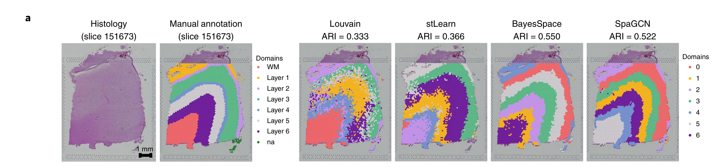

实际的效果

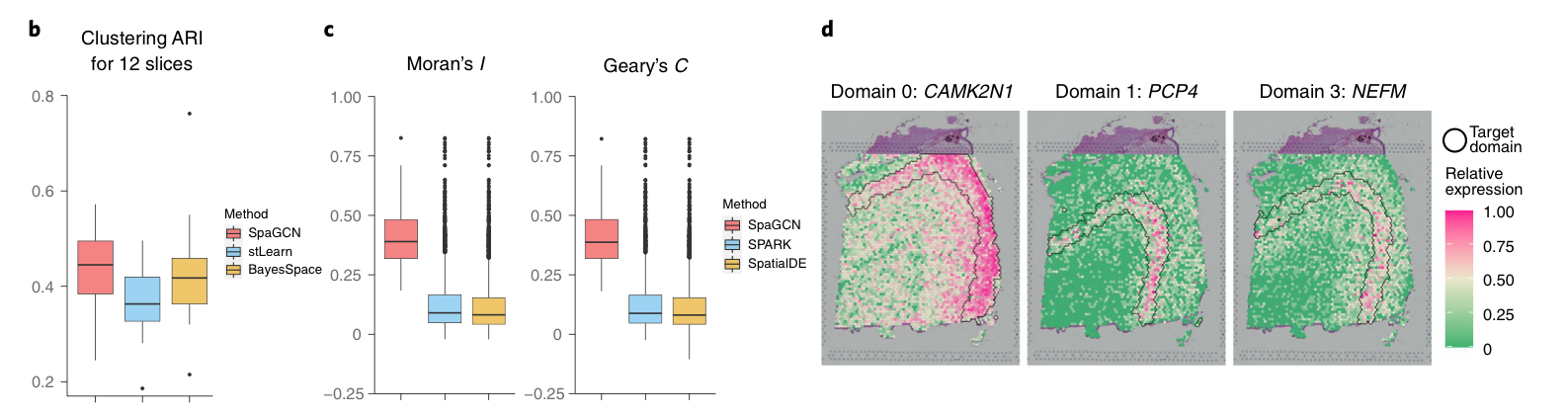
b 图表示了考虑到所有 12 个 slices 后 the median ARI is 0.36 for stLearn, 0.42 for BayesSpace and 0.45 for SpaGCN.

In total, SpaGCN detected 67 SVGs, with 53 of them being specific to domain 5, which corresponds to white matter.Patterns of SVGs for other domains are not very clear.

These results indicate that gene expression profiles of spots from white matter are distinct from spots in the neuronal layers, while gene expression differences among the six neuronal layers are much smaller and more difficult to distinguish using individual marker genes.

White Matter（白质） 是大脑和脊髓中的一种组织，主要由髓鞘包裹的神经纤维（轴突）组成，其颜色在肉眼观察下呈现白色。白质的主要功能是通过神经纤维连接大脑不同区域和大脑与脊髓之间的信号通路，起到信息传递的作用。

d 图: For three out of the six neuronal layers, SpaGCN detected a single SVG to mark that region.

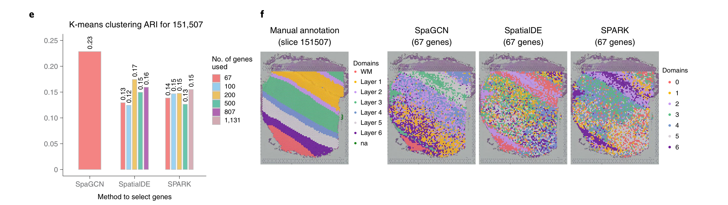
这是在检测它的 downstream（下游）的影响，利用 K-means 对它进行聚类。我们发现增加 SVGs 的数量并没有提高 SoatialDE 和 SPARK 的 ARIs 的值，证明了 the lack of spatial patterns for genes detected by SPARK and SpatialDE.

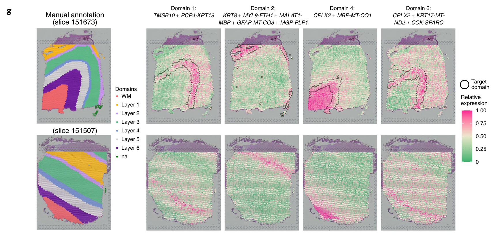
SpaGCN was able to find domain-specific meta genes.
这个 meta 基因貌似并没有准确的定义，暂时将它理解为：指在特定组织区域、细胞群体或功能性领域中表现出独特表达模式的一组基因。

例如 FTH1,MBP,MT-CO3 and PLP1 是 Depleted gene

Depleted Genes（耗减基因）指的是在某个特定条件、组织区域、细胞类型或实验处理下，表达水平显著低于其他条件或区域的基因。

Enriched Genes（富集基因）是指在特定条件、样本组、组织区域或细胞类型中，基因的表达水平显著高于其他条件、区域或细胞类型的基因。

# Application to mouse posterior (后面的) brain 10x Visium data

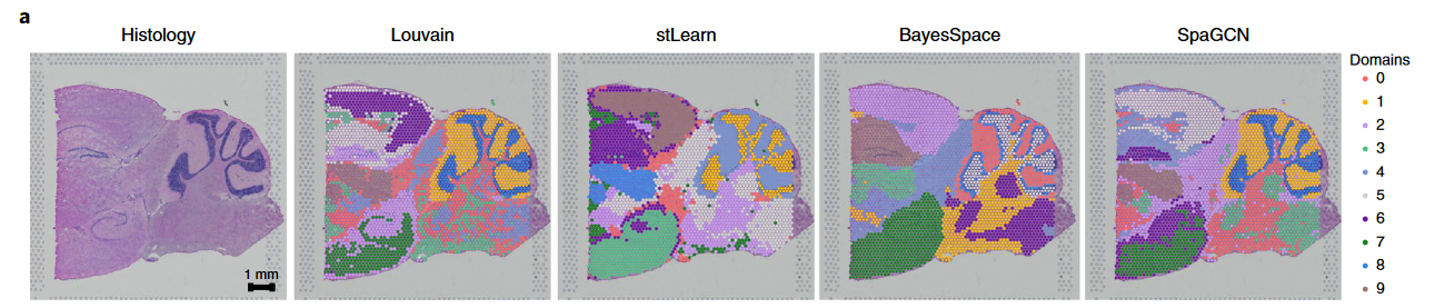
Louvain's clustering is similar to stLearn, BayesSpace and SpaGCN, but the spatial domains detected by the latter three methods are more spatially contiguous due too their ability to account for spatial dependency of gene expression.

图 b: we performed subclustering analysis for spots in domain 5 detected by SpaGCN, which corresponds to the cortex.

图 c: The subdomians detected by SpaGCN agree well with the Allen Brain Institute reference atlas diagram of the mouse cortex.
可以看的出来 SpaGCN 在此例中的拟合效果比其它几种方法都要好

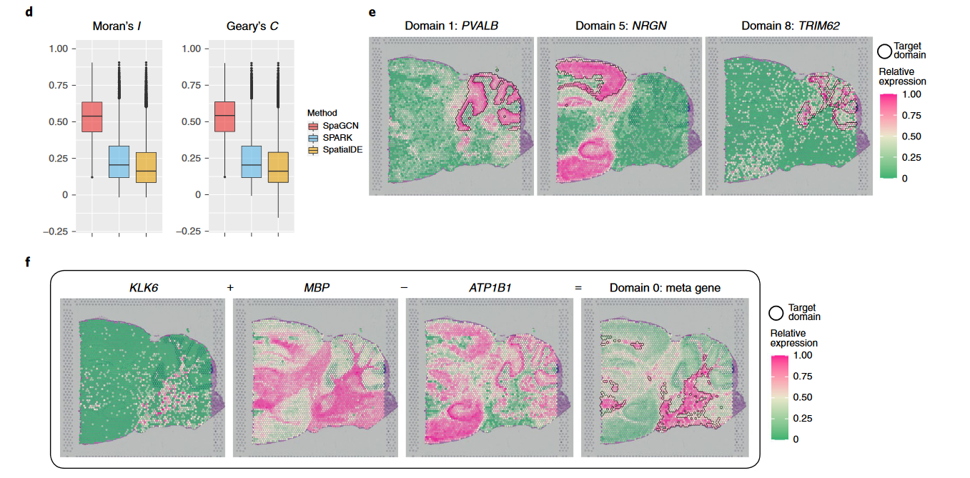
d 图：Multiple domain adaptive filtering criteria implemented in SpaGCN allow it to eliminate false positive SVGs and ensure all detected SVGs have clear spatial expression patterns

e 图: Illustrate how the filtering in SpaGCN works, we use domains 1, 5 and 8 as an example.

对于 domain1 和 8，即使它们相邻，但是 SpaGCN 仍能很好的将它们区分出来。

domains 5 and 7, which would be contiguous in a three-dimensional(3D) reconstruction, are artifactually separated as a result of how the section was cut.

f 图: An example to show how SpaGCN can create informative meta genes to mark a spatial domain.

SpaGCN only identified four SVGs for dimain 0. However, we reason that a meta gene, formed by the combination of multiple genes, may better reveal spatial patterns than any single genes.

说实话不是很能理解这个所谓的 meta gene，即使能够很好的表现，那么依据呢？为什么这几个合一起就更好，是巧合还是什么其它的因素？

好吧，结果紧接着这篇文章就解释了原因。我感觉这个和之前学过的因子分析有点像，先聚合在一起，然后根据结果 “瞎编” 理由:

KLK6 and MBP are considered as positive markers because they are highly expressed insome spots in domain 0, whereas ATP1B1 is considered a negative marker as it is mainly expressed in regions other than domain 0.

Previous studies studies have shoen that KLK6 and MBP expression is restricted to oligodendrocytes, while ATP1B1 is mainly expressed in neurons and astrocytes. This resonates with the fact that domain 0 represents white matter which is dominated by oligodendrocytes and has few neuronal cell bodies.

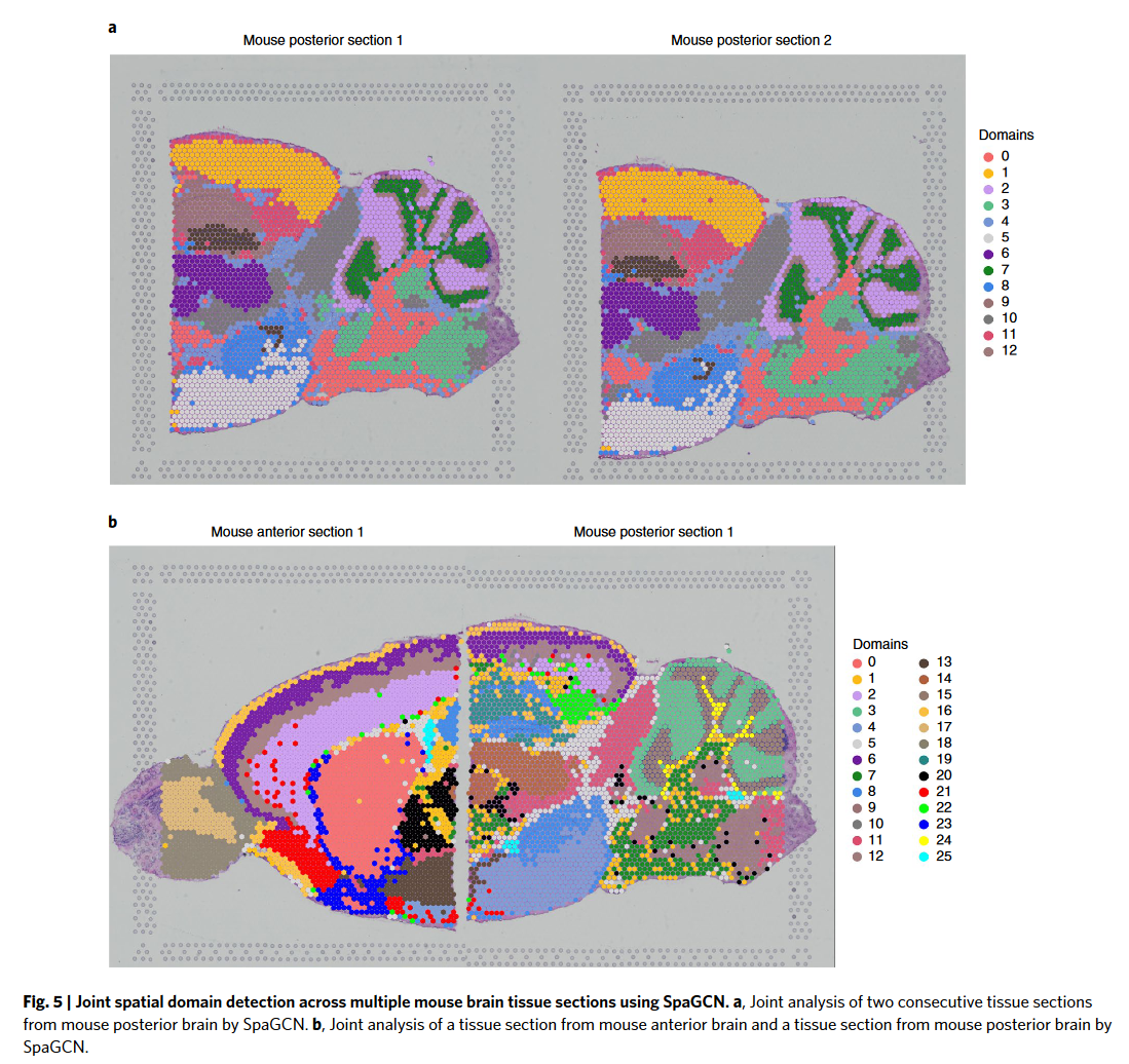
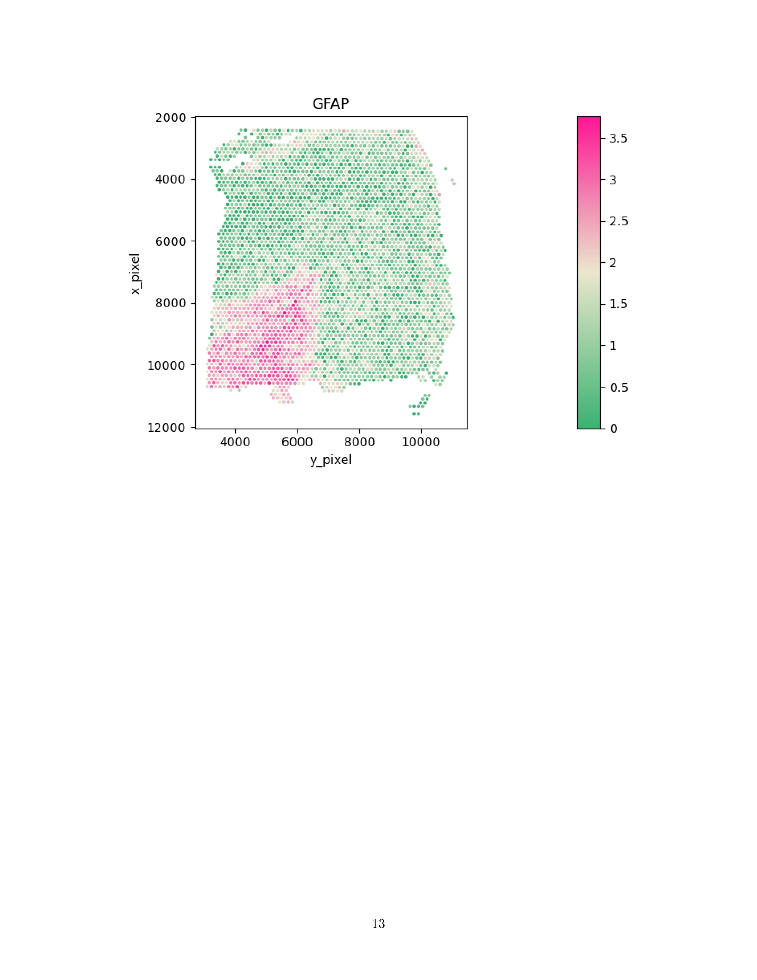
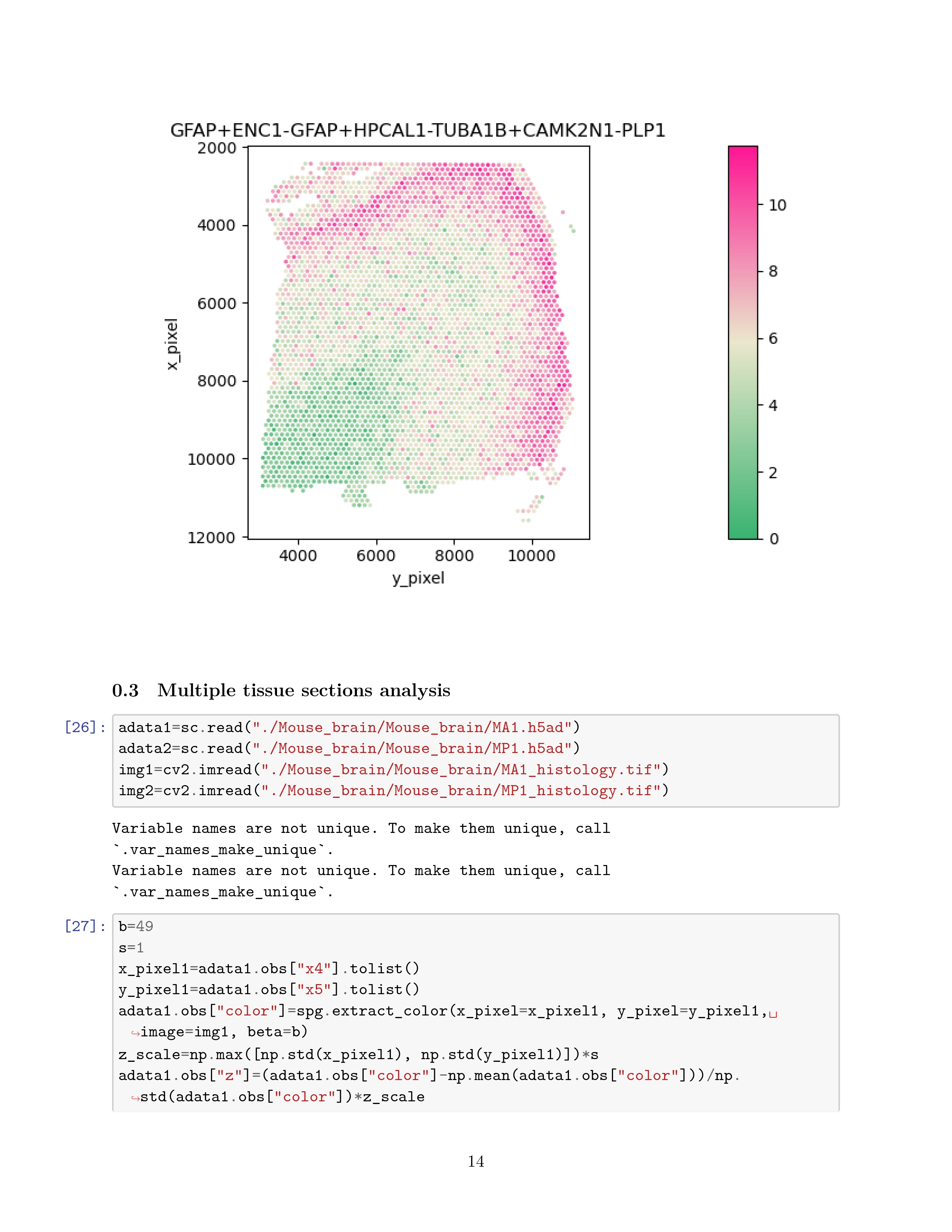
SpaGCN can also jointly analyze multiple tissue sections.

SpaGCN was able to infer cluster correspondence between the two tissue sections.

Using the modified coordinates as input, SpaGCN was able to produce clustering results that reflect the shared layer structure in the anterior and posterior brain.

# Application to mouse visual cortex STARmap data

STARmap data 是更精密但更少的数据，这里是为了体现 SpaGCN 的泛用性。

This example demonstrates that SpaGCN utilizes spatial information more efficiently than BayesSpace and HMRF.

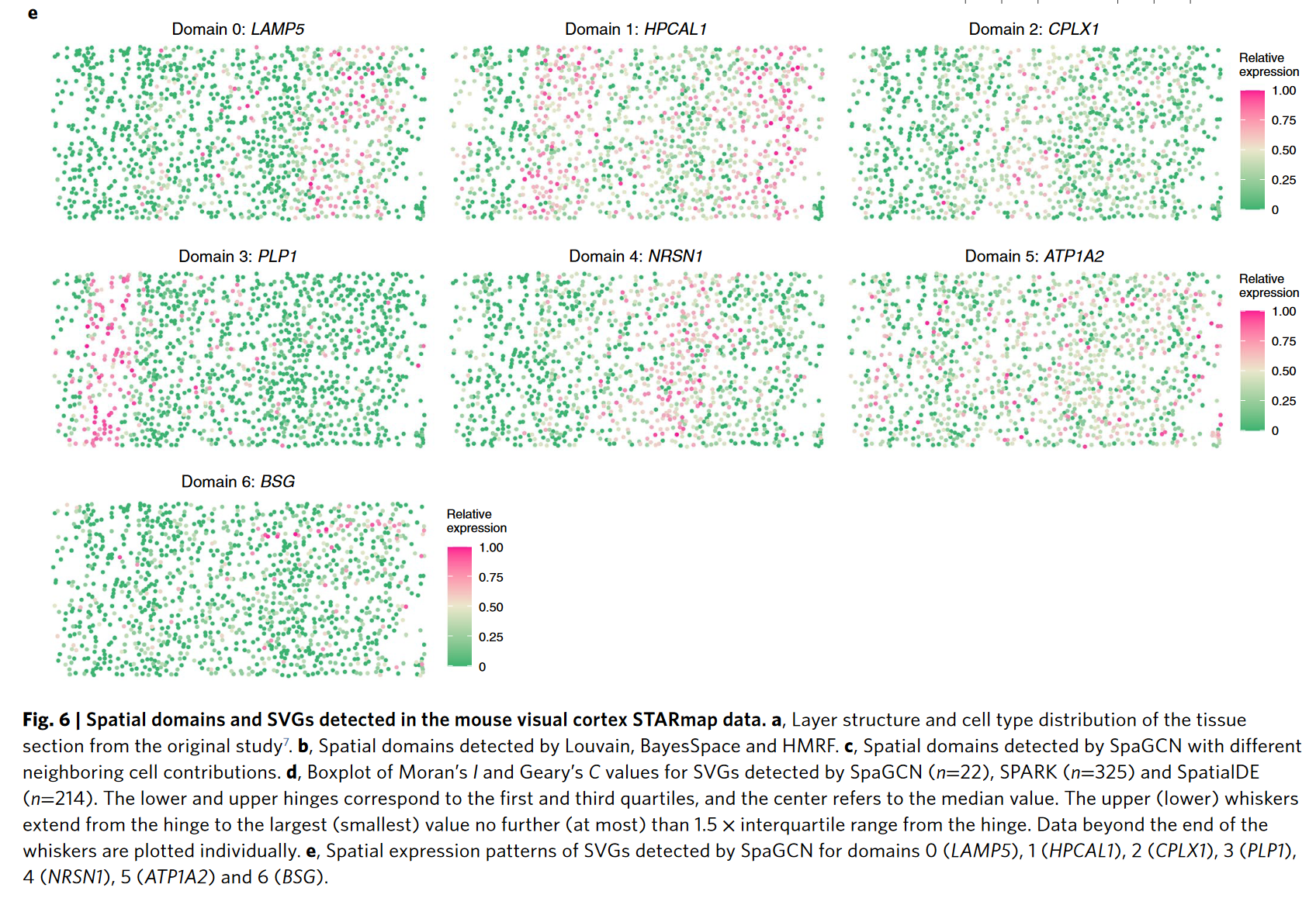
这是对于 SVG 的检测

# Discussion

A limitation of SpaGCN is that the spatial domain detection is mainly driven by gene expression, which may lead to the discrepeancy between the detected domains and the underlying tissue anatomical structure.

Another limitation of SpaGCN is the lack of separation of spatial variation and cell type variation in gene expression patterns for the detected SVGs.

Further cell type-specific gene expression needs to be estimated to tease out the contribution of cell types and spatial location in gene expression variation.

# Methods

# Data prepocessing

The spatial gene expression data are stored in an $N\times D$ matrix of unique molecular identifier(UMI) counts with $N$ spots and $D$ genes, along with the $(x,y)$ two-dimensional(2D) spatial coordinates of each spot.

The gene expression values in each spot are normalized such that the UMI count for each gene is divided by the total UNI count across all genes in a given spot, multiplied by 10000, and the transformed to a natrual log scale.

UMI count 是指通过使用 Unique Molecular Identifiers（UMI）技术，在高通量测序中每个特定分子的出现次数。UMI count 的主要目的是在测序数据中，统计每个独特分子（基因、转录本等）在样本中的 “真实” 丰度，而不是依赖于传统的计数方式（即直接根据测序读段的数量来估算丰度），因为 UMI count 可以消除由于 PCR 扩增带来的重复性偏差。
UMI count 的工作原理
标签引入：在实验过程中，每个目标分子（如 mRNA 或 DNA 片段）都会与一个独特的 UMI 标签序列一起被捕获和扩增。这些 UMI 标签通常在目标序列的两端加上。
测序：在高通量测序时，UMI 标签和目标序列都会被读取。
去重与计数：在数据分析阶段，所有带有相同 UMI 标签的读段被归为同一组，并且这组只计为一个分子。因此，每个 UMI 标签代表一个独立的分子，而不是由 PCR 扩增产生的多个重复。
UMI count：最终，UMI count 表示每个特定分子在样本中出现的次数，帮助准确估算每个基因或转录本的表达水平。
UMI count 的应用
基因表达量：在转录组学研究中，UMI count 可以准确地计算基因的表达水平，避免了由于 PCR 扩增带来的误差。
单细胞 RNA 测序：在单细胞测序中，每个细胞的 RNA 分子都会被标记上独特的 UMI 标签，从而可以有效地消除测序误差和扩增偏差，确保对每个单细胞的基因表达量进行精准估算。
突变检测：在基因组学和癌症研究中，UMI count 可以帮助准确检测和定量低频突变或稀有变异，避免了由于 PCR 扩增引入的重复导致的假阳性。
总的来说，UMI count 是一种有效的计数方式，使得基于测序的数据更加精确和可靠，尤其在处理复杂样本和高丰度与低丰度分子并存的情况下，能显著提高数据的准确性。

# Conversion of SRT data into graph-structured data

SpaGCN converts the gene expression and histology image data into a weighted undirected graph, $G(V,E)$ .each vertex $v\in V$ represents a spot and every two vertices in $V$ are connected via an edge with a specified weight.

spage2vec employed a graph-based approach, but with the goal of clustering messenger RNA molecules.

# Calculation of distance between two vertices

The distance between any two vertics $u$ and $v$ in the graph reflects the relative similarity of the two corresponding spots.

This distance is determined by two factors:

the physical location of spot $u$ and $v$ in the tissue slice
the corresponding histology information of these two spots.

consider two spots tobe close if and only if :

physically close
similar histological features as shown in the histology image

pixel coordinates : $(\mathcal{x}_{pv},\mathcal{y}_{pv})$

SpaGCN draws a square centered on $(\mathcal{x}_{pv},\mathcal{y}_{pv})$ containing $50 \times 50$ pixels and calculates the mean color value for the RGB channels, $(r_v,g_v,b_v)$

\begin{equation} \mathcal{z_v} = \frac{r_v \times V_r + g_v \times V_g + b_v \times V_b}{V_r + V_g + V_b} \end{equation}

where $V_r$ = variance( $r_v$ ) ...

SpaGCN rescales $\mathcal{z_v}$ as

\begin{equation} \mathcal{z_v^*}= \frac{z_v-\mu_z}{\sigma_z} \times max(\sigma_x,\sigma_y) \times s \end{equation}

where $\mu_z$ is the mean of $z_v$ $\sigma_x,\sigma_y,\sigma_z$ are the standard deviations of $\mathcal{x}_{v},\mathcal{y}_{v},\mathcal{z}_{v}$ , and $s$ is a scaling factor.

Euclidean distance between every two spots $u$ and $v$ is calculated as:

\begin{equation} d(u,v) = \sqrt{(x_u-x_v)^2+(y_u-y_v)^2+(z_u^*-z_v^*)^2} \end{equation}

# Calculation of weight for each edge and construction of graph

The graph structure G is stored in an $N\times N$ adjacency matrix $A=[w(u,v)]$ , where the edge weight between spot u and spot v is defined as

\begin{equation} w(u,v) = exp(-\frac{d(u,v)^2}{2l^2}) \end{equation}

这里是类似于机器学习里面的高斯核

The hyperparameter $l$ , also known as the characteristic length scale, determines how rapidly the weight decays as a function of distance. A similar function has been employed in SpatialDE.

For spot $v$ , the corresponding row sum of $A-I$ , denoted by $a_v$ , can be interpreted as the relative contribution of other spots to its gene expression.

# Graph convolutional layer

对于 X 矩阵，使用 PCA，取前 50 个主成分作为输入。然后使用 graph convolutional network。

the graph convolutional layer can be written as:

\begin{equation} f(X,A) = \delta(AXB), \end{equation}

$X$ is the $N \times 50$ embedding matrix obtained from PCA, B is a $50 \times 50$ matrix representing filter parameters of the convolutional layer, and $\delta(\cdot)$ is a nonlinear activation function such as ReLU.

说实话这个粗暴的取前 50 个主成分也算是节省了运算的时间。然而之前我在跑一个数据集较小的数据时，SpaGCN 直接就报错了，因为在那个数据集中只有 32 维。

原文写到：Through graph convolution, SpaGCN has aggregated the gene expression information according to the edge weights specified in G. The output of this layer is an aggregated matrix that includes information on gene expression, spatial location and histology.

我大概拿 chatgpt 跑了个关于 spage2vec 的介绍：

以下是将空间转录组学数据转化为向量嵌入的步骤：
数学符号和定义
空间转录组学数据：假设我们有一个空间转录组学数据集，这个数据集可以表示为一组节点 $\mathcal{V}={v_1, v_2, \dots, v_n}$ ，其中每个节点 $v_i$ 代表一个空间位置。
基因表达矩阵：对于每个空间位置 $v_i$ ，我们有一个高维基因表达向量 $\mathbf{x}_i\in\mathbb{R}^d$ ，其中 $d$ 是基因的数量。所有节点的基因表达数据可以构成一个基因表达矩阵 $\mathbf{X}=[\mathbf{x}_1, \mathbf{x}_2, \dots, \mathbf{x}_n]^\top \in \mathbb{R}^{n \times d}$ 。
空间邻接关系：我们假设相邻的空间位置在图中通过一条边相连，用图 $G=(\mathcal{V}, \mathcal{E})$ 表示空间邻接关系，其中 $\mathcal{E}$ 是边的集合。可以根据物理位置或其他准则（例如距离）定义边的存在，邻接矩阵 $\mathbf{A} \in \mathbb{R}^{n \times n}$ 表示图的结构， $A_{ij}=1$ 表示节点 $v_i$ 和 $v_j$ 相连，反之 $A_{ij} = 0$ 。
SpaGE2vec 的数学过程
图卷积层的定义：
我们通过图卷积神经网络（Graph Convolutional Network, GCN）对基因表达矩阵 $\mathbf{X}$ 和邻接矩阵 $\mathbf{A}$ 进行图卷积操作。
具体来说，图卷积可以表示为：
\begin{equation} \mathbf{H}^{(l+1)} = \sigma\left(\tilde{\mathbf{D}}^{-\frac{1}{2}} \tilde{\mathbf{A}} \tilde{\mathbf{D}}^{-\frac{1}{2}} \mathbf{H}^{(l)} \mathbf{W}^{(l)}\right) \end{equation}
$\tilde{\mathbf{A}} = \mathbf{A} + \mathbf{I}$ 为加上自连接后的邻接矩阵；
$\tilde{\mathbf{D}}$ 是 $\tilde{\mathbf{A}}$ 的度矩阵；
$\mathbf{H}^{(l)}$ 是第 $l$ 层的节点特征矩阵，初始时 $\mathbf{H}^{(0)} = \mathbf{X}$ ；
$\mathbf{W}^{(l)}$ 是该层的权重矩阵；
$\sigma$ 是激活函数（例如 ReLU）。
嵌入表示：
经过多层图卷积后，我们可以得到每个节点的低维嵌入向量表示 $\mathbf{Z} = \mathbf{H}^{(L)} \in \mathbb{R}^{n \times k}$ ，其中 $L$ 是图卷积的层数， $k$ 是嵌入的维度。
这个矩阵 $\mathbf{Z}$ 是我们要得到的嵌入结果，每一行 $\mathbf{z}_i \in \mathbb{R}^k$ 表示节点 $v_i$ 的低维嵌入。
嵌入的聚类和分析：
在得到嵌入矩阵 $\mathbf{Z}$ 后，我们可以使用聚类算法（如 k-means）对这些向量进行聚类，将具有相似基因表达和空间特征的节点归为一类。
通过聚类结果，我们可以发现组织中不同区域的基因表达特征差异。
例子分析
假设我们在肿瘤组织上使用 SpaGE2vec，得到以下结果：
每个空间点的嵌入 $\mathbf{z}_i$ 可以被分为几类，分别代表肿瘤中心、肿瘤边缘、健康组织等区域。
使用 t-SNE 或 UMAP 对嵌入结果 $\mathbf{Z}$ 进行二维可视化后，我们发现这些区域在嵌入空间中彼此分离开来。

但吊诡的是，这里面倒是的的确确使用了 gene expression 的数据，那么 SpaGCN 呢？后面看代码印证一下吧。

# Spatial domain identification by clustering

空间域的概念: SpaGCN employs an unsupervised clustering algorithm iteratively to cluster the spots into different spatial domains. Each cluster identified from this analysis is considered to be a spatial domain, which contains spots that are coherent in gene expression and histology.

首先确定一个初始的中心，这里是利用 Louvain 算法。我感觉这个 Louvain 算法和 K-means 有点像，都是要确定一下分类的数量和初始点。分类的数量（也就是 domain 的数量）取决于我们是否知道 the number of domains in the tissue. 如果不知道就 vary the resolution parameter from 0.2 to 1.0 and select the resolution that gives the highest Silhouette score.

Louvain 算法是一种常用的社区检测算法，用于发现复杂网络中的社区结构。分辨率参数是一个重要的超参数，用于控制社区检测的粒度，通常由符号 $\gamma$ 表示

当 $\gamma = 1$ ,Louvain 算法的标准形式，社区检测的结果通常是最平衡的。

当 $\gamma < 1$ ,Louvain 算法倾向于检测更大的社区，因为较小的社区合并的可能性更大。

当 $\gamma > 1$ ,Louvain 算法倾向于检测更小的社区，因为较大的社区会被拆分成更小的社区。

下面的公式我并没有看懂。这个公式是为了衡量每个 spot $i$ 的 embedded point $h_i$ 和 centroid $\mu_j$ 对于每个类 $j$ 的距离：

\begin{equation} q_{ij} = \frac{(1+h_i-\mu_j^2)^{-1}}{\sum_{j' = 1}^{K} (1+h_i-\mu_{j'}^2)^{-1}} \end{equation}

可以被诠释为将细胞 i 分类给细胞 j 的概率

然后文章定义了一个 auxiliary target distribution $P$ based on q_

\begin{equation} p_{ij} = \frac{q_{ij}^2 / {\sum^{N}_{i=1}} q_{ij}}{\sum_{j^{\prime}}^{K}(q_{ij^{\prime}}^2 / {\sum^{N}_{i=1}q_{ij^{\prime}}})} \end{equation}

然后又解释这个能对高置信度分配的点赋予更大的权重，并对每个簇中心在整体损失函数中的贡献进行归一化，以防止大簇扭曲隐藏特征空间。

这句话的意思是，在某些模型或算法中，存在两种不同的分配方式：

软分配 $q_{ij}$ ：
- 软分配通常表示一个模糊的或连续的分配关系。在聚类或分类问题中，软分配可以用于描述一个数据点 $i$ 属于簇 $j$ 的概率，而不是硬性地将其分配给一个特定的簇。通常，软分配值会在 0 和 1 之间，表示一个数据点属于某个簇的 “程度”。
- 例如，在高斯混合模型（Gaussian Mixture Model, GMM）中，软分配 $q_{ij}$ 表示数据点 $i$ 属于簇 $j$ 的概率，且该概率随着模型的训练不断调整。
辅助分配 $p_{ij}$ ：
- 辅助分配通常是用于辅助计算的一种参考分配，可能并不直接用于最终的分类或聚类结果。它可能是模型中的一个中间变量，或者是用来约束某些条件的辅助信息。
- 辅助分配通常用来调节或优化模型，例如在变分推断中，辅助分配 $p_{ij}$ 可能是通过某种假设或者近似推断得到的，旨在帮助模型更好地收敛或更精确地估计分布。

然后定义损失函数 Kullback-Leibler (KL) divergence loss
KL 散度可以理解为：如果使用分布 $Q$ 来近似分布 $P$ ，会有多少信息损失。具体来说，KL 散度衡量了使用 $Q$ 来表示 $𝑃$ 时的平均信息损失或不匹配程度。

\begin{equation} L = KL(P||Q) = \displaystyle\sum^{N}_{i=1}\displaystyle\sum^{K}_{j=1}p_{ij}log\frac{p_{ij}}{q_{ij}} \end{equation}

通过利用随机梯度下降的方法最小化 $L$ 的值训练模型

这一个板块看着倒逻辑通畅，实际上每一步都理解不了为什么要这么去实现，后面再研究一下。

// 这里研究出来了，它本质上是使用了 DEC (Deep Embedded Clustering) 的方法

参考网站

结合这个文章一看，我们大胆推测这个 SpaGCN 里面针对 q 的公式怕不是写错了？应该是：

\begin{equation} q_{ij} = \frac{(1+(h_i-\mu_j)^2)^{-1}}{\sum_{j' = 1}^{K} (1+(h_i-\mu_{j'})^2)^{-1}} \end{equation}

对应着代码

1
2
3

q = 1.0 / ((1.0 + torch.sum((x.unsqueeze(1) - self.mu)**2, dim=2) / self.alpha) + 1e-8)
        q = q**(self.alpha+1.0)/2.0
        q = q / torch.sum(q, dim=1, keepdim=True)

而且抽象的是他这里直接写了指数为 - 1，然而原本论文的公式为：

\begin{equation} q_{ij} = \frac{(1+(h_i-\mu_j)^2/\alpha)^{-\frac{\alpha+1}{2}}}{\sum_{j' = 1}^{K} (1+(h_i-\mu_j)^2/\alpha)^{-\frac{\alpha+1}{2}}} \end{equation}

他自己设定的 $\alpha = 0.2$ 然而论文里面却直接默认 $\alpha = 1$

也不知道是什么情况

# Detection of SVGs

原文提到要设立一个半径去找邻居，也没具体介绍，这里我根据代码写一下原理：

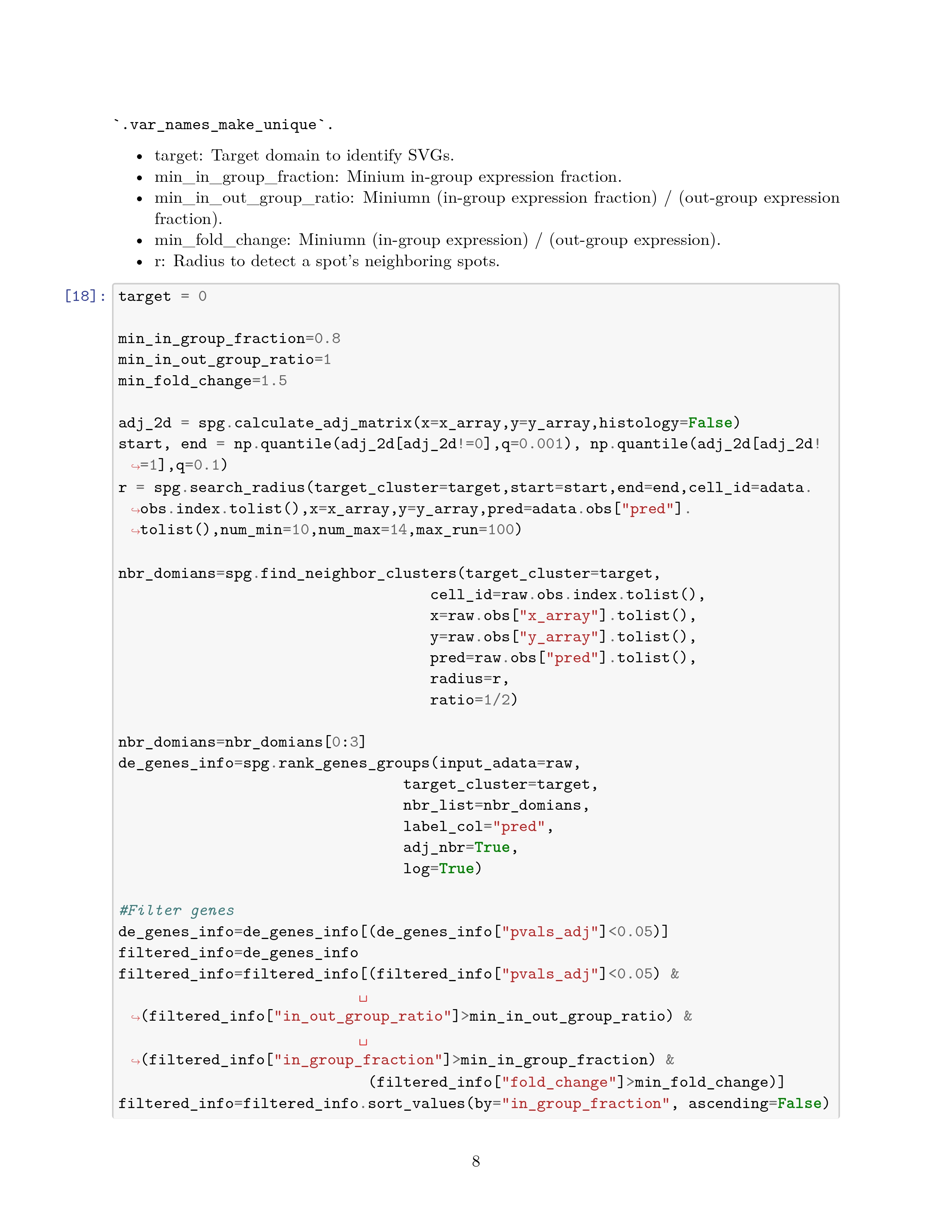
首先根据 spot 之间的距离，通过邻接矩阵取非零值排序，对于在分位点 0.1% 和 10% 的分位数作为搜索 radius 的 start 和 end
接着去计算每个细胞在指定的 radius 所包含细胞邻居数量的平均值，我们希望这个平均值在 8-15 之间，这个应该是经验值。得到的 radius 便是所求的半径。

这里直接去看原文吧，提到了一些准则，后面会在这里补充一下什么是 DE analysis，什么是 Wilcoxon rank-sum test. 主要是使用了这两种方法

差异表达分析（DE Analysis）的核心原理是通过比较两组（或多组）样本中基因表达的分布差异，识别在不同条件下显著变化的基因。这涉及数据预处理、统计建模和显著性评估等多个步骤，核心原理如下：

# 1. 数据来源与表示

差异表达分析以基因表达矩阵为输入，矩阵的结构如下：

行：基因。
列：样本。
值：基因在某样本中的表达量（通常是计数值，如 RNA-Seq 的 read counts，或已标准化的表达值，如 TPM、FPKM）。

例如：

基因 / 样本	样本 1（对照）	样本 2（实验）	样本 3（对照）	样本 4（实验）
GeneA	50	100	45	95
GeneB	200	210	195	220

# 2. 数据预处理

为了消除技术或生物学噪声对结果的影响，差异表达分析需要先对数据进行预处理：

去除低表达基因：
- 低表达的基因贡献的信息有限，可能会引入噪声。
- 通常的阈值是：在至少一组样本中计数值大于某个值（如 10）。
归一化（Normalization）：
- 由于不同样本测序深度不同，需要对表达量进行归一化。
- 常见方法：
  - TPM/FPKM/RPKM：标准化为每百万读数的基因表达值。
  - DESeq2 的 size factor。
  - EdgeR 的 TMM（Trimmed Mean of M-values）。
对数变换：
- 由于基因表达分布往往是偏态的（如负二项分布），对数变换可使数据更接近正态分布，便于后续统计分析。

# 3. 差异表达的统计模型

差异表达分析的核心是比较两组样本中基因表达的差异。这需要统计模型来评估表达变化是否显著。

# （1）假设检验

每个基因进行一次假设检验，设定零假设 $H_0$ 和备择假设 $H_1$ ：

$H_0$ ：该基因在两组样本中的表达量无显著差异。
$H_1$ ：该基因在两组样本中的表达量有显著差异。

# 检验方法：

t 检验：
- 假设表达值符合正态分布。
- 适用于小样本但表达值已标准化的数据。
- 不适合原始 RNA-Seq 计数值。
非参数检验（如 Wilcoxon 检验）：
- 无需假设数据分布，适合较为广泛的场景。
基于离散分布的模型（RNA-Seq 数据常用）：
- RNA-Seq 数据是计数型，且存在离散性和过度离散性（overdispersion）。
- 常用方法：
  - EdgeR：基于负二项分布建模。
  - DESeq2：基于广义线性模型（GLM），以负二项分布校正过度离散性。

# 关键统计量：

Fold Change（FC）：
- 表示基因在实验组和对照组之间的表达倍数变化。
- 常用对数形式： $\text{log2FC} = \log_2(\text{实验组均值}/\text{对照组均值})$ 。
p-value：
- 根据统计检验方法计算的显著性水平。
- 较小的 p-value 表明表达差异可能显著。

# （2）多重检验校正

DE 分析涉及多个基因（通常上万个）的独立假设检验，需控制整体的假阳性率。

问题：直接使用 p-value 会导致大量假阳性（type I error）。
方法：
- 使用 FDR（False Discovery Rate）校正，常用算法：
  - Benjamini-Hochberg 方法。
  - Bonferroni 校正（较为严格）。

结果是校正后的 p-value，称为 adjusted p-value 或 q-value。

# 4. 差异基因筛选

根据以下标准筛选差异表达基因（DEGs）：

Fold Change（FC）：
- 通常设定阈值，如 $|\text{log2FC}| > 1$ 。
p-value 或 Adjusted p-value：
- 常用阈值： $\text{q-value} < 0.05$ 。

例如：

基因	log2FC	Adjusted p-value
GeneA	2.5	0.001
GeneB	-1.2	0.02

# 5. 可视化与结果解释

# （1）火山图（Volcano Plot）

x 轴：log2 Fold Change。
y 轴：-log10 (p-value)。
用不同颜色标注显著的差异表达基因。

# （2）热图（Heatmap）

显示差异基因在各样本间的表达模式。
可聚类分析样本和基因之间的关系。

# 6. 后续分析

功能富集分析：
- 通过 Gene Ontology (GO)、KEGG 等数据库，解析差异基因的生物学功能。
信号通路分析：
- 分析差异基因对信号通路的影响。
验证：
- 通过实验方法（如 qPCR）验证筛选出的关键基因。

总结：DE 分析的核心原理是基于统计模型和检验，评估基因在不同样本组间的表达差异。通过合理的数据预处理、显著性评估和多重检验校正，可以高效筛选出生物学意义显著的差异表达基因，为后续研究提供关键线索。
Wilcoxon 秩和检验（Wilcoxon Rank-Sum Test），也叫 Mann-Whitney U 检验，是一种非参数统计检验方法，用于比较两组数据的分布是否有显著差异。它特别适用于以下情况：

数据不满足正态分布假设。
样本量较小。
数据是有序的（ordinal），但可能不是连续的。

# 1. 应用场景

Wilcoxon 秩和检验常用于以下问题：

比较两组数据的中位数是否不同。
检测两组数据是否来自相同的分布。

# 2. 原理

该检验基于数据的秩（rank），而不是原始数值，从而对异常值和数据分布的要求不敏感。

# （1）假设

零假设 $H_0$ ：两组数据的分布相同。
备择假设 $H_1$ ：
- 双尾检验：两组数据的分布不同。
- 单尾检验：一组数据的分布显著大于或小于另一组。

# （2）步骤

合并数据并排序：
- 将两组数据合并，根据大小为每个值分配一个秩（rank）。
- 如果有重复值，赋予它们相同的秩，计算平均秩。
计算秩和：
- 分别计算两组数据的秩和（sum of ranks）。
计算检验统计量：
- $U_1 = R_1 - \frac{n_1(n_1+1)}{2}$ $U_{1} = R_{1} - \frac{n _{1} ( n _{1} + 1 )}{2}$
  U_2 = R_2 - \frac{n_2(n_2+1)}
  - $R_1, R_2$ ：两组数据的秩和。
  - $n_1, n_2$ ：两组数据的样本量。
- 检验统计量 $U = \min(U_1, U_2)$ 。
计算 p 值：
- 根据 $U$ 值和两组样本量，从查表或通过正态分布近似计算 p 值。

# 3. 示例

假设有两组数据：

组 1（对照）：[85, 90, 78]
组 2（实验）：[88, 92, 85]

# 步骤 1：合并并排序

数据排序后：

值	78	85	85	88	90	92
秩	1	2.5	2.5	4	5	6

# 步骤 2：计算秩和

组 1（对照，85, 90, 78）： $R_1 = 1 + 2.5 + 5 = 8.5$
组 2（实验，88, 92, 85）： $R_2 = 2.5 + 4 + 6 = 12.5$

# 步骤 3：计算 $U$ 值

$U_1 = R_1 - \frac{n_1(n_1+1)}{2} = 8.5 - \frac{3 \cdot (3+1)}{2} = 8.5 - 6 = 2.5$
$U_2 = R_2 - \frac{n_2(n_2+1)}{2} = 12.5 - \frac{3 \cdot (3+1)}{2} = 12.5 - 6 = 6.5$
$U = \min(U_1, U_2) = \min(2.5, 6.5) = 2.5$

# 步骤 4：查表得 p 值

根据 $U = 2.5$ 和 $n_1 = n_2 = 3$ ，查表或计算 p 值。
如果 $p < 0.05$ ，拒绝 $H_0$ 。

# 4. 优点

对数据分布无要求（非正态分布可用）。
对极值不敏感。
适合小样本分析。

# 5. 限制

对于非常大的样本，非参数方法的效能可能不如参数方法（如 t 检验）。
假设两组数据是独立的，且度量尺度至少是有序的。
无法提供基于具体差异大小的效应量估计。

# Detection of spatially variable meta genes

每次迭代的公式

\begin{equation} log(meta\_gene_{t+1}) = log(meta\_gene_t) + log(gene_{t+}) - log(gene_{t-}) + C_t \end{equation}

原本我以为这个 meta genes 没啥用，结果发现构造它的方法也十分巧妙合乎逻辑，其实主要的逻辑就是处理上一个板块若是没有出现 SVGs 的 domain 该怎么处理。

# Evaluation of SVGs using Moran'sI and Geary's statics

这个板块直接去看 benchmarking 的那篇文章的解释即可

接下来就是代码的部分了。

# 代码

好恶心

由于不理解不会的太多以至于我不知道该怎么记了，先大致先从 Clustering 和 SVGs 两个板块来记录吧，最后再记录一下实际使用 SpaGCN 的步骤。

# Clustering

# 原理性的东西

class SpaGCN(object):
    def __init__(self):
        super(SpaGCN, self).__init__()
        self.l=None

    def set_l(self, l):
        self.l=l

    def train(self,adata,adj, 
            num_pcs=50, 
            lr=0.005,
            max_epochs=2000,
            weight_decay=0,
            opt="admin",
            init_spa=True,
            init="louvain", #louvain or kmeans
            n_neighbors=10, #for louvain
            n_clusters=None, #for kmeans
            res=0.4, #for louvain
            tol=1e-3):
        self.num_pcs=num_pcs
        self.res=res
        self.lr=lr
        self.max_epochs=max_epochs
        self.weight_decay=weight_decay
        self.opt=opt
        self.init_spa=init_spa
        self.init=init
        self.n_neighbors=n_neighbors
        self.n_clusters=n_clusters
        self.res=res
        self.tol=tol
        assert adata.shape[0]==adj.shape[0]==adj.shape[1]
        pca = PCA(n_components=self.num_pcs)
        if issparse(adata.X):
            pca.fit(adata.X.A)
            embed=pca.transform(adata.X.A)
        else:
            pca.fit(adata.X)
            embed=pca.transform(adata.X)
        ###------------------------------------------###
        if self.l is None:
            raise ValueError('l should not be set before fitting the model!')
        adj_exp=np.exp(-1*(adj**2)/(2*(self.l**2)))
        #----------Train model----------
        self.model=simple_GC_DEC(embed.shape[1],embed.shape[1])
        self.model.fit(embed,adj_exp,lr=self.lr,max_epochs=self.max_epochs,weight_decay=self.weight_decay,opt=self.opt,init_spa=self.init_spa,init=self.init,n_neighbors=self.n_neighbors,n_clusters=self.n_clusters,res=self.res, tol=self.tol)
        self.embed=embed
        self.adj_exp=adj_exp

    def predict(self):
        z,q=self.model.predict(self.embed,self.adj_exp)
        y_pred = torch.argmax(q, dim=1).data.cpu().numpy()
        # Max probability plot
        prob=q.detach().numpy()
        return y_pred, prob

p: Percentage of total expression contributed by neighborhoods. 也对应着论文中的 the average of $a_v$ across all spots
l: Parameter to control p.
res: 是用来控制在 Louvain 中聚类的分辨率的，需要先用算法去生成这个值，然后能得到对应的能生成具体对应区块数目的 res 值

输入中 adata，adj 是由下面的代码得到的，全部都可以由 h5ad 数据得到：

adata = sc.read_h5ad(f'{datadir}/osmfish.h5ad')
adata.obs['x_pixel']=adata.obsm['spatial'][:,0]
adata.obs['y_pixel']=adata.obsm['spatial'][:,1]

x_pixel=adata.obs["x_pixel"].tolist()
y_pixel=adata.obs["y_pixel"].tolist()

adj=spg.calculate_adj_matrix(x=x_pixel,y=y_pixel, histology=False)

self 指的是实例本身，也便是我们利用这个 class 创建出来的实例。

然后便是调用 model 里面的函数。
model：

class simple_GC_DEC(nn.Module):
    def __init__(self, nfeat, nhid, alpha=0.2):
        super(simple_GC_DEC, self).__init__()
        self.gc = GraphConvolution(nfeat, nhid)
        self.nhid=nhid
        #self.mu determined by the init method
        self.alpha=alpha

    def forward(self, x, adj):
        x=self.gc(x, adj)
        q = 1.0 / ((1.0 + torch.sum((x.unsqueeze(1) - self.mu)**2, dim=2) / self.alpha) + 1e-8)
        q = q**(self.alpha+1.0)/2.0
        q = q / torch.sum(q, dim=1, keepdim=True)
        return x, q

    def loss_function(self, p, q):
        def kld(target, pred):
            return torch.mean(torch.sum(target*torch.log(target/(pred+1e-6)), dim=1))
        loss = kld(p, q)
        return loss

    def target_distribution(self, q):
        #weight = q ** 2 / q.sum(0)
        #return torch.transpose((torch.transpose(weight,0,1) / weight.sum(1)),0,1)e
        p = q**2 / torch.sum(q, dim=0)
        p = p / torch.sum(p, dim=1, keepdim=True)
        return p

    def fit(self, X,adj,  lr=0.001, max_epochs=5000, update_interval=3, trajectory_interval=50,weight_decay=5e-4,opt="sgd",init="louvain",n_neighbors=10,res=0.4,n_clusters=10,init_spa=True,tol=1e-3):
        self.trajectory=[]
        if opt=="sgd":
            optimizer = optim.SGD(self.parameters(), lr=lr, momentum=0.9)
        elif opt=="admin":
            optimizer = optim.Adam(self.parameters(),lr=lr, weight_decay=weight_decay)

        features= self.gc(torch.FloatTensor(X),torch.FloatTensor(adj))
        #----------------------------------------------------------------        
        if init=="kmeans":
            print("Initializing cluster centers with kmeans, n_clusters known")
            self.n_clusters=n_clusters
            kmeans = KMeans(self.n_clusters, n_init=20)
            if init_spa:
                #------Kmeans use exp and spatial
                y_pred = kmeans.fit_predict(features.detach().numpy())
            else:
                #------Kmeans only use exp info, no spatial
                y_pred = kmeans.fit_predict(X)  #Here we use X as numpy
        elif init=="louvain":
            print("Initializing cluster centers with louvain, resolution = ", res)
            if init_spa:
                adata=sc.AnnData(features.detach().numpy())
            else:
                adata=sc.AnnData(X)
            sc.pp.neighbors(adata, n_neighbors=n_neighbors)
            sc.tl.louvain(adata,resolution=res)
            y_pred=adata.obs['louvain'].astype(int).to_numpy()
            self.n_clusters=len(np.unique(y_pred))
        #----------------------------------------------------------------
        y_pred_last = y_pred
        self.mu = Parameter(torch.Tensor(self.n_clusters, self.nhid))
        X=torch.FloatTensor(X)
        adj=torch.FloatTensor(adj)
        self.trajectory.append(y_pred)
        features=pd.DataFrame(features.detach().numpy(),index=np.arange(0,features.shape[0]))
        Group=pd.Series(y_pred,index=np.arange(0,features.shape[0]),name="Group")
        Mergefeature=pd.concat([features,Group],axis=1)
        cluster_centers=np.asarray(Mergefeature.groupby("Group").mean())
        
        self.mu.data.copy_(torch.Tensor(cluster_centers))
        self.train()
        for epoch in range(max_epochs):
            if epoch%update_interval == 0:
                _, q = self.forward(X,adj)
                p = self.target_distribution(q).data
            if epoch%10==0:
                print("Epoch ", epoch) 
            optimizer.zero_grad()
            z,q = self(X, adj)
            loss = self.loss_function(p, q)
            loss.backward()
            optimizer.step()
            if epoch%trajectory_interval == 0:
                self.trajectory.append(torch.argmax(q, dim=1).data.cpu().numpy())

            #Check stop criterion
            y_pred = torch.argmax(q, dim=1).data.cpu().numpy()
            delta_label = np.sum(y_pred != y_pred_last).astype(np.float32) / X.shape[0]
            y_pred_last = y_pred
            if epoch>0 and (epoch-1)%update_interval == 0 and delta_label < tol:
                print('delta_label ', delta_label, '< tol ', tol)
                print("Reach tolerance threshold. Stopping training.")
                print("Total epoch:", epoch)
                break


    def fit_with_init(self, X,adj, init_y, lr=0.001, max_epochs=5000, update_interval=1, weight_decay=5e-4,opt="sgd"):
        print("Initializing cluster centers with kmeans.")
        if opt=="sgd":
            optimizer = optim.SGD(self.parameters(), lr=lr, momentum=0.9)
        elif opt=="admin":
            optimizer = optim.Adam(self.parameters(),lr=lr, weight_decay=weight_decay)
        X=torch.FloatTensor(X)
        adj=torch.FloatTensor(adj)
        features, _ = self.forward(X,adj)
        features=pd.DataFrame(features.detach().numpy(),index=np.arange(0,features.shape[0]))
        Group=pd.Series(init_y,index=np.arange(0,features.shape[0]),name="Group")
        Mergefeature=pd.concat([features,Group],axis=1)
        cluster_centers=np.asarray(Mergefeature.groupby("Group").mean())
        self.mu.data.copy_(torch.Tensor(cluster_centers))
        self.train()
        for epoch in range(max_epochs):
            if epoch%update_interval == 0:
                _, q = self.forward(torch.FloatTensor(X),torch.FloatTensor(adj))
                p = self.target_distribution(q).data
            X=torch.FloatTensor(X)
            adj=torch.FloatTensor(adj)
            optimizer.zero_grad()
            z,q = self(X, adj)
            loss = self.loss_function(p, q)
            loss.backward()
            optimizer.step()

    def predict(self, X, adj):
        z,q = self(torch.FloatTensor(X),torch.FloatTensor(adj))
        return z, q

forward 函数对应着

\begin{equation} q_{ij} = \frac{(1+(h_i-\mu_j)^2)^{-1}}{\sum_{j' = 1}^{K} (1+(h_i-\mu_{j'})^2)^{-1}} \end{equation}

这也是上面提到过的
可以看到他显式的定义了 alpha=0.2，说明我们上面的猜测也是没错的。

loss_function 对应着

\begin{equation} L = KL(P||Q) = \displaystyle\sum^{N}_{i=1}\displaystyle\sum^{K}_{j=1}p_{ij}log\frac{p_{ij}}{q_{ij}} \end{equation}

target_distribution 对应着：

\begin{equation} p_{ij} = \frac{q_{ij}^2 / {\sum^{N}_{i=1}} q_{ij}}{\sum_{j^{\prime}}^{K}(q_{ij^{\prime}}^2 / {\sum^{N}_{i=1}q_{ij^{\prime}}})} \end{equation}

这里最不好理解的就是 features 是什么东西，以下是它的解释，方便后面来查阅：

# 图卷积层的计算过程

图卷积层（GC）通常执行以下步骤：

特征聚合：对于每个节点，将其特征与邻居节点的特征进行加权求和。
线性变换：通过一个线性变换（通常是矩阵乘法）将聚合后的特征转换为新的特征表示。
激活函数：通常还会应用一个激活函数（如 ReLU）来引入非线性。

# 具体计算步骤

假设我们有一个简单的图数据集，并且已经定义了一个图卷积层，以下是一个完整的示例：

# 导入必要的模块

import torch
import torch.nn as nn
import torch.nn.functional as F
import numpy as np
import pandas as pd

# 定义一个简单的图卷积层

class GraphConvolution(nn.Module):
    def __init__(self, in_features, out_features):
        super(GraphConvolution, self).__init__()
        self.weight = nn.Parameter(torch.FloatTensor(in_features, out_features))
        self.reset_parameters()
    
    def reset_parameters(self):
        nn.init.xavier_uniform_(self.weight)
    
    def forward(self, X, adj):
        support = torch.mm(X, self.weight)
        output = torch.spmm(adj, support)
        return output

# 创建一个简单的数据集

# 创建一个简单的特征矩阵
X = np.array([[1, 2, 3], [4, 5, 6], [7, 8, 9]])

# 创建一个简单的邻接矩阵
adj = np.array([[0, 1, 0], [1, 0, 1], [0, 1, 0]])

# 创建模型实例并处理数据

# 创建图卷积层实例
gc = GraphConvolution(in_features=3, out_features=3)

# 将特征矩阵和邻接矩阵转换为 PyTorch 张量
X_tensor = torch.FloatTensor(X)
adj_tensor = torch.FloatTensor(adj)

# 通过图卷积层处理特征
features = gc(X_tensor, adj_tensor)

# 将结果从 PyTorch 张量转换为 NumPy 数组
features_np = features.detach().numpy()

# 打印结果
print("Original Features:\n", X)
print("Transformed Features:\n", features_np)

# 具体计算过程

特征矩阵 X 和邻接矩阵 adj ：
- X 的形状为 (3, 3) ，表示 3 个节点，每个节点有 3 个特征。
- adj 的形状为 (3, 3) ，表示节点之间的连接关系。
初始化权重矩阵 self.weight ：
- self.weight 是一个形状为 (3, 3) 的矩阵，通过 Xavier 初始化方法初始化。
特征聚合：
- 首先，将输入特征矩阵 X 与权重矩阵 self.weight 进行矩阵乘法，得到支持矩阵 support 。
- support = torch.mm(X, self.weight)
线性变换：
- 然后，将支持矩阵 support 与邻接矩阵 adj 进行稀疏矩阵乘法，得到输出特征矩阵 output 。
- output = torch.spmm(adj, support)
激活函数（可选）：
- 在这个例子中，我们没有应用激活函数，但在实际应用中，通常会应用 ReLU 等激活函数。

# 示例计算

假设初始化后的权重矩阵 self.weight 如下：

self.weight = torch.FloatTensor([
    [0.1, 0.2, 0.3],
    [0.4, 0.5, 0.6],
    [0.7, 0.8, 0.9]
])

# 计算支持矩阵 `support`

1	support = torch.mm(X_tensor, self.weight)

具体计算如下：

X_tensor = [[1, 2, 3],
            [4, 5, 6],
            [7, 8, 9]]

self.weight = [[0.1, 0.2, 0.3],
               [0.4, 0.5, 0.6],
               [0.7, 0.8, 0.9]]

support = X_tensor @ self.weight

计算结果：

support = [[1 * 0.1 + 2 * 0.4 + 3 * 0.7, 1 * 0.2 + 2 * 0.5 + 3 * 0.8, 1 * 0.3 + 2 * 0.6 + 3 * 0.9],
           [4 * 0.1 + 5 * 0.4 + 6 * 0.7, 4 * 0.2 + 5 * 0.5 + 6 * 0.8, 4 * 0.3 + 5 * 0.6 + 6 * 0.9],
           [7 * 0.1 + 8 * 0.4 + 9 * 0.7, 7 * 0.2 + 8 * 0.5 + 9 * 0.8, 7 * 0.3 + 8 * 0.6 + 9 * 0.9]]

support = [[2.4, 3.2, 4.0],
           [6.0, 8.0, 10.0],
           [9.6, 12.8, 16.0]]

# 计算输出特征矩阵 `output`

1	output = torch.spmm(adj_tensor, support)

具体计算如下：

adj_tensor = [[0, 1, 0],
              [1, 0, 1],
              [0, 1, 0]]

support = [[2.4, 3.2, 4.0],
           [6.0, 8.0, 10.0],
           [9.6, 12.8, 16.0]]

output = adj_tensor @ support

计算结果：

output = [[0 * 2.4 + 1 * 6.0 + 0 * 9.6, 0 * 3.2 + 1 * 8.0 + 0 * 12.8, 0 * 4.0 + 1 * 10.0 + 0 * 16.0],
          [1 * 2.4 + 0 * 6.0 + 1 * 9.6, 1 * 3.2 + 0 * 8.0 + 1 * 12.8, 1 * 4.0 + 0 * 10.0 + 1 * 16.0],
          [0 * 2.4 + 1 * 6.0 + 0 * 9.6, 0 * 3.2 + 1 * 8.0 + 0 * 12.8, 0 * 4.0 + 1 * 10.0 + 0 * 16.0]]

output = [[6.0, 8.0, 10.0],
          [12.0, 16.0, 20.0],
          [6.0, 8.0, 10.0]]

# 最终结果

1 2	print("Original Features:\n", X) print("Transformed Features:\n", features_np)

输出可能如下：

Original Features:
 [[1 2 3]
 [4 5 6]
 [7 8 9]]
Transformed Features:
 [[ 6.0  8.0 10.0]
 [12.0 16.0 20.0]
 [ 6.0  8.0 10.0]]

# 解释

原始特征 X ：
- 输入特征矩阵 X 的形状为 (3, 3) ，表示 3 个节点，每个节点有 3 个特征。
变换后的特征 features ：
- 经过图卷积层处理后， features 变成了一个新的特征矩阵，形状仍然是 (3, 3) ，但内容已经包含了图结构的信息。
- 例如，第一个节点的新特征 [6.0, 8.0, 10.0] 是通过聚合第一个节点的特征及其邻居节点的特征得到的。
数据类型转换：
- features 最初是一个 PyTorch 张量。
- 通过 detach() 方法从计算图中分离张量，返回一个新的张量，不再记录任何梯度信息。
- 通过 numpy() 方法将 PyTorch 张量转换为 NumPy 数组，方便后续的数据处理和分析。

# 总结

图卷积层通过特征聚合和线性变换将输入特征矩阵 X 转换为新的特征表示 features ，这些新的特征表示包含了图结构的信息。希望这个详细的解释能帮助你更好地理解和使用图卷积层的计算过程。

需要注意的是，如果像我们的代码没有显式的定义 weight 的值，它会自动用 xavier 来定义一个。这对应论文中的 B 矩阵。

class GraphConvolution(Module):
    """
    Simple GCN layer, similar to https://arxiv.org/abs/1609.02907
    """

    def __init__(self, in_features, out_features, bias=True):
        super(GraphConvolution, self).__init__()
        self.in_features = in_features
        self.out_features = out_features
        self.weight = Parameter(torch.FloatTensor(in_features, out_features))
        #self.weight 是通过 nn.Parameter 定义的，并且在 reset_parameters 方法中使用了 nn.init.xavier_uniform_ 方法进行初始化。这意味着 self.weight 的值会被 Xavier 均匀分布初始化方法随机初始化。
        if bias:
            self.bias = Parameter(torch.FloatTensor(out_features))
        else:
            self.register_parameter('bias', None)
        self.reset_parameters()

    def reset_parameters(self):
        stdv = 1. / math.sqrt(self.weight.size(1))
        self.weight.data.uniform_(-stdv, stdv)
        if self.bias is not None:
            self.bias.data.uniform_(-stdv, stdv)

    def forward(self, input, adj):
        support = torch.mm(input, self.weight)
        output = torch.spmm(adj, support)
        if self.bias is not None:
            return output + self.bias
        else:
            return output

    def __repr__(self):
        return self.__class__.__name__ + ' (' \
               + str(self.in_features) + ' -> ' \
               + str(self.out_features) + ')'

上面是论文中的代码定义的卷积层，可以看到它是如何定义的。

# 1. `self` 是什么？为什么 `self(X, adj)` 可以前向传播？

self 是当前模型实例：
- 在 Python 的类定义中， self 代表类的实例。在 PyTorch 中， self 通常是 torch.nn.Module 的子类实例，即一个模型对象。
为什么可以调用 self(X, adj) ？
- 这是因为在定义模型类时，我们重载了 nn.Module 的 __call__ 方法（继承自 PyTorch 的 nn.Module ）。
- 当执行 self(X, adj) 时，会自动调用模型的 forward 方法，这在模型设计中是标准行为：
  1
  2
  3
  def forward(self, x, adj):
  # 前向传播的逻辑
  ...
- 所以 self(X, adj) 是 self.forward(X, adj) 的简写，直接执行前向传播。

# 2. 为什么 `loss` 是一个数，却可以调用 `loss.backward()` ？底层逻辑是什么？

# `loss` 的值和张量计算图

loss 是一个标量张量：
- loss 是通过 loss_function(p, q) 计算得来的，其值是一个单一标量张量，例如形状为 torch.Size([]) 。
- PyTorch 会为所有涉及 p 和 q 的计算构建动态计算图，记录每一步计算及其操作（加法、乘法等）。

# `backward()` 的作用

当调用 loss.backward() 时：
- PyTorch 沿着计算图，从 loss 的值开始，计算其对每个参数的梯度。
- 这些梯度会存储到模型的参数（如 self.gc 和 self.mu ）的 grad 属性中。

# 如何支持梯度计算？

计算图的构建依赖 PyTorch 的张量操作，所有张量都默认 requires_grad=False 。
只有模型参数（如 self.parameters() 返回的张量）设置了 requires_grad=True ，PyTorch 才会在计算图中记录这些张量的操作，进而支持梯度计算。

# 3. 为什么可以执行 `optimizer.step()` ？ `optimizer` 默认操作的是谁？

# `optimizer` 是如何绑定模型参数的？

优化器初始化时，我们传入了 self.parameters() ：

1	optimizer = optim.SGD(self.parameters(), lr=lr, momentum=0.9)

self.parameters() 是一个生成器，包含模型中所有可训练参数（即 requires_grad=True 的张量），如 self.gc 和 self.mu 。
优化器会记录这些参数，并在调用 optimizer.step() 时，更新这些参数的值。

# `optimizer.step()` 的作用

在调用 loss.backward() 后，参数的梯度存储在每个参数的 grad 属性中。
optimizer.step() 使用这些梯度，根据优化算法（如 SGD 或 Adam）更新参数值：
- SGD 更新公式： param = param - lr * grad
- Adam 等高级算法会对梯度进行一些额外的修正。

# 4. `self.train()` 训练了什么？

self.train() 的作用：
- 它不会直接 “训练” 模型，而是将模型切换到训练模式。
- PyTorch 的 nn.Module 有两种模式： train() 和 eval() 。
  - 在 train() 模式下，某些层（如 Dropout 和 BatchNorm ）会启用特定的训练行为。
  - 在 eval() 模式下，这些层的行为会发生变化（如 Dropout 禁用、 BatchNorm 使用固定统计值）。
模型训练本质：
- 训练实际上由反向传播和优化器更新参数实现：
  1. 前向传播计算输出；
  2. 计算损失；
  3. 调用 loss.backward() 计算梯度；
  4. 调用 optimizer.step() 更新参数。

# 总结

self 是模型实例，调用 self(X, adj) 本质是调用模型的 forward 方法。
loss 是一个标量张量，它的计算图记录了所有依赖操作， loss.backward() 会计算所有参数的梯度。
optimizer.step() 更新的是绑定到优化器的模型参数，这些参数通过 self.parameters() 显式指定。
self.train() 设置模型为训练模式，实际训练逻辑由前向传播、反向传播和优化器更新完成。

上面的代码都是 simple 的部分，还有一个正常版本，多了 ReLu 和 dropout，设立了两层卷积层。这里就不赘述了，大体思路是一样的。

# SVGs

# 原理性的东西

其实反倒这里没什么好说的了，具体实现的东西和论文里面差不多，可以记录几个自己认为值得记录的几处：

1
2
3

nbr_num = [(k, v) for k, v in nbr_num.items() if v > (ratio * cluster_num[k])]

nbr_num.sort(key=lambda x: -x[1])

这里面是通过 nbr_num.items () 取出键值对

lambda x: -x[1] 是一个匿名函数，接受一个二元组 x 作为输入，返回 -x[1] ，即二元组的第二个元素的负值。

其实具体就是把论文中提到的给实现了，没什么好说的

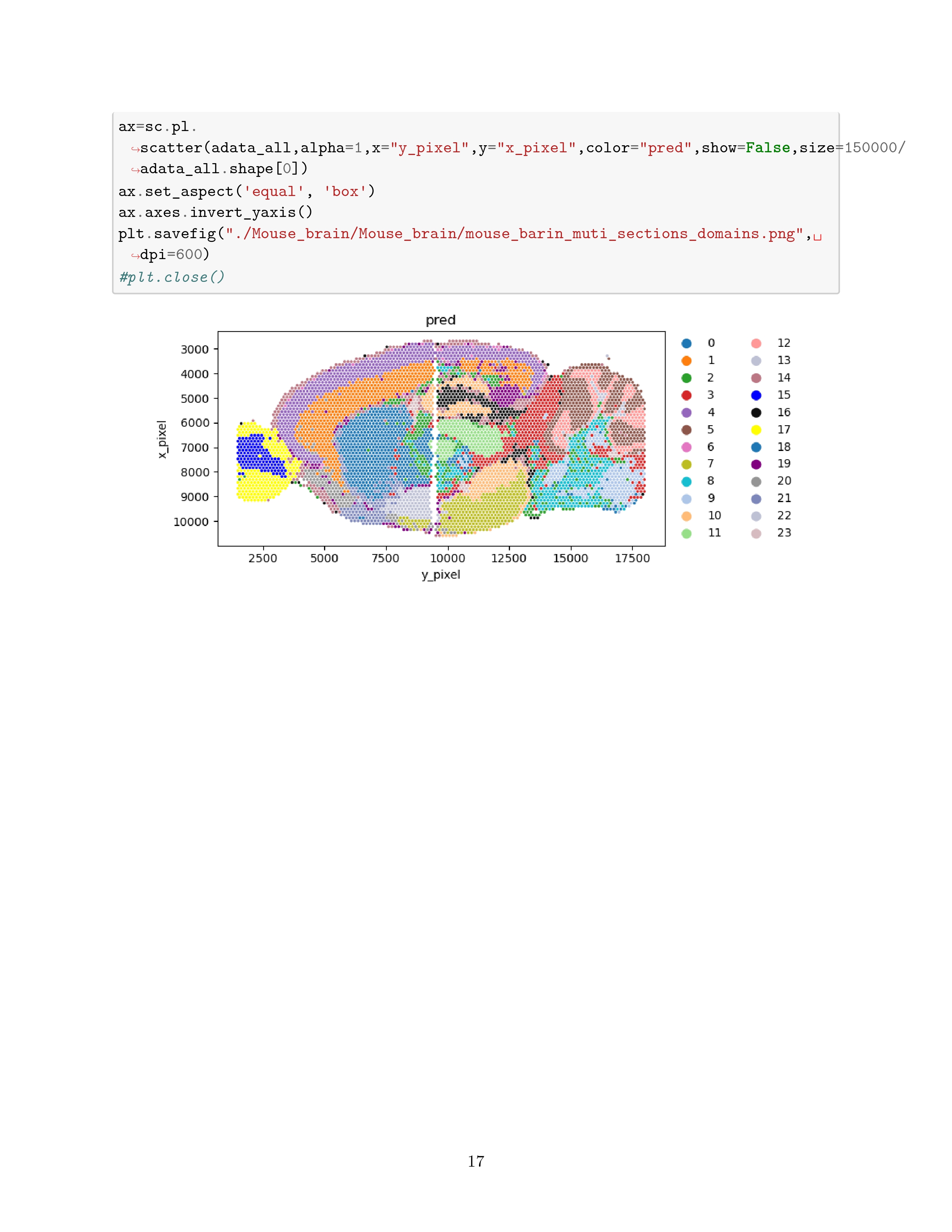
# 实际使用

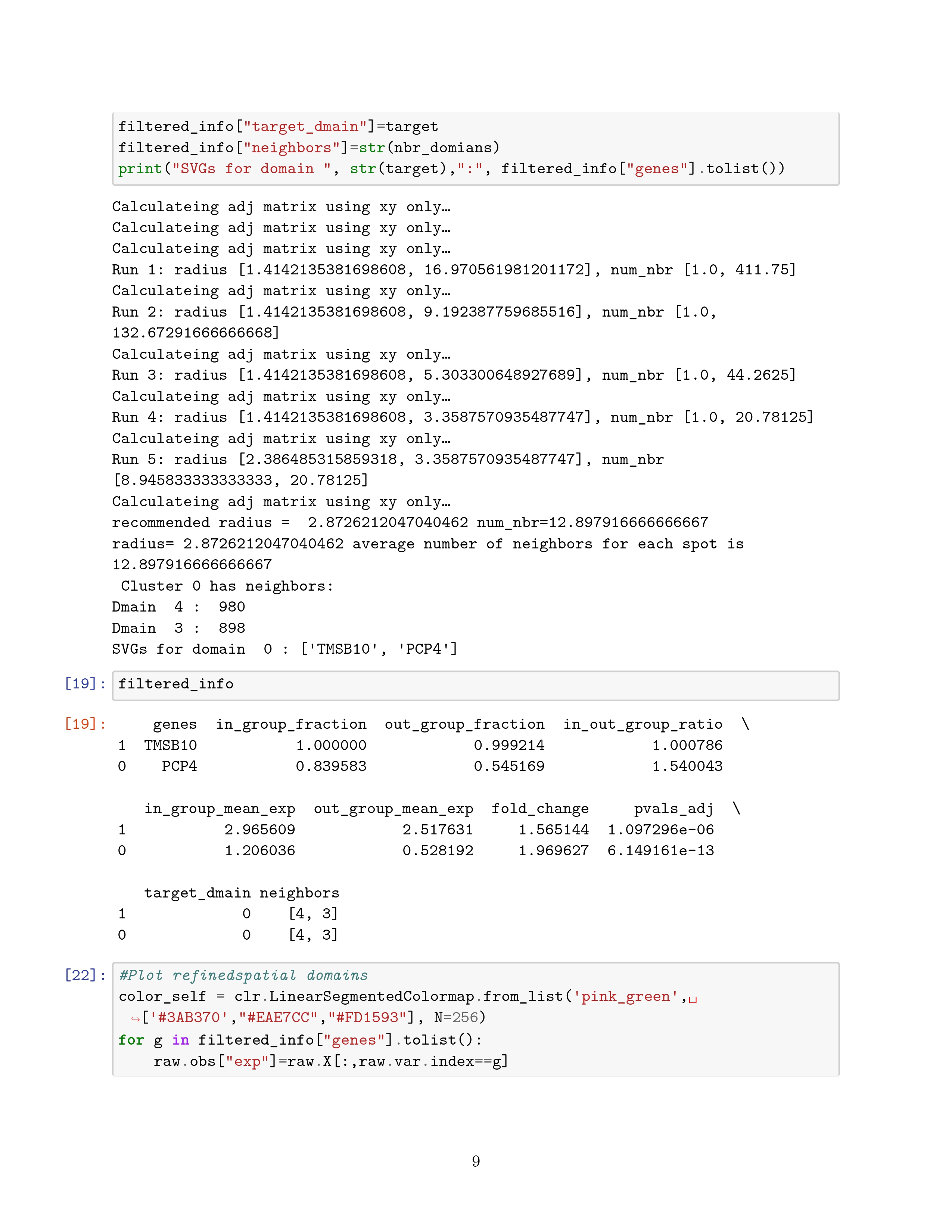
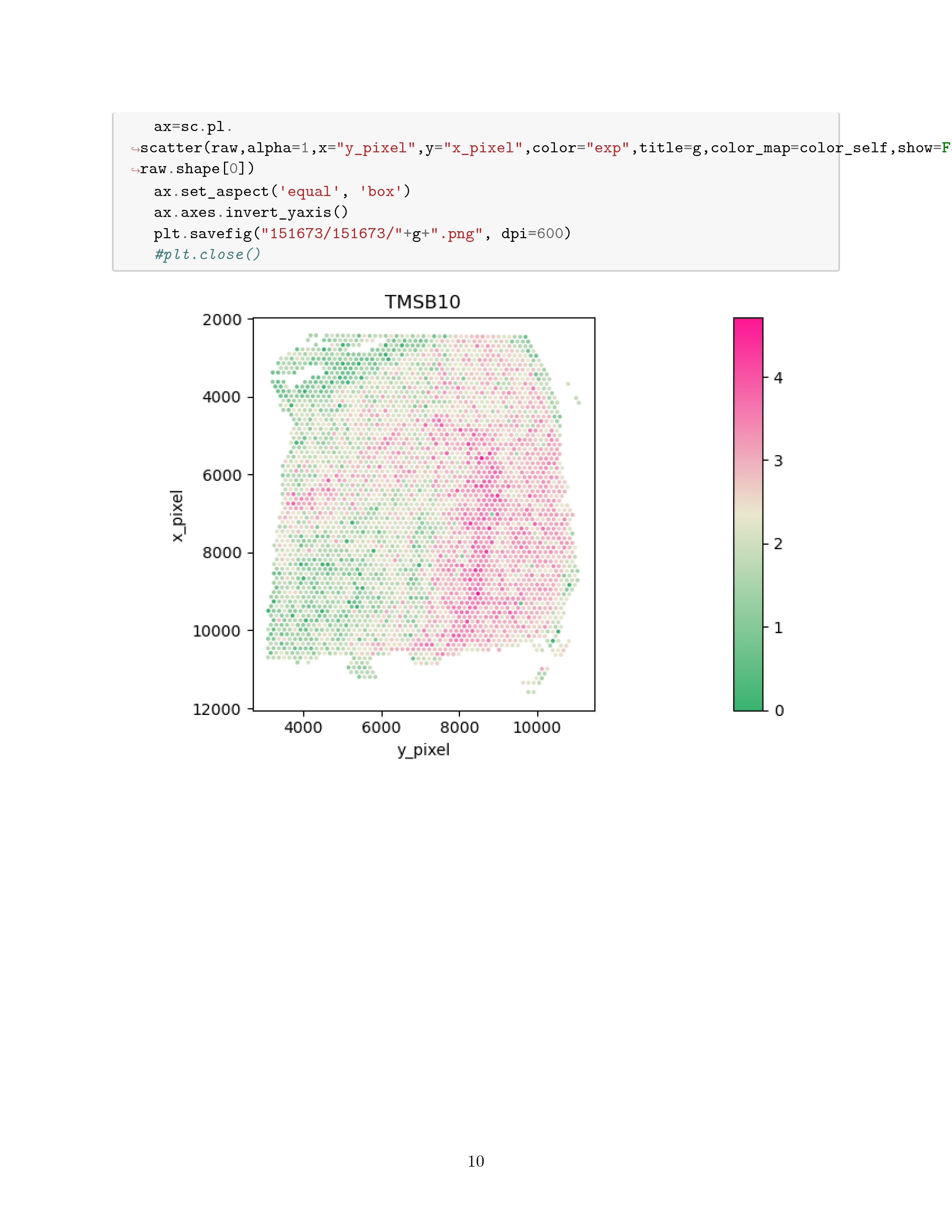
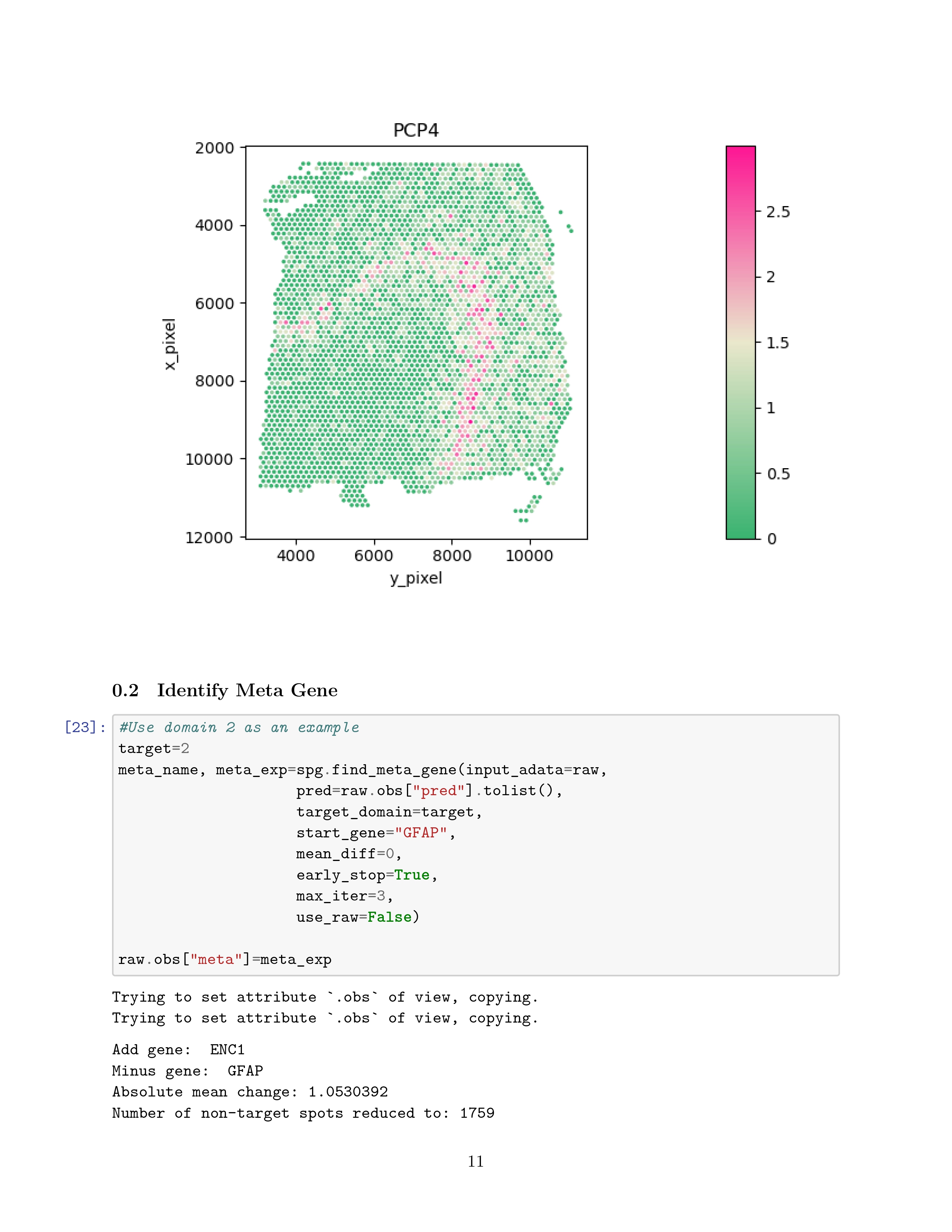
这里就具体记录一下自己复现过程遇到的问题吧
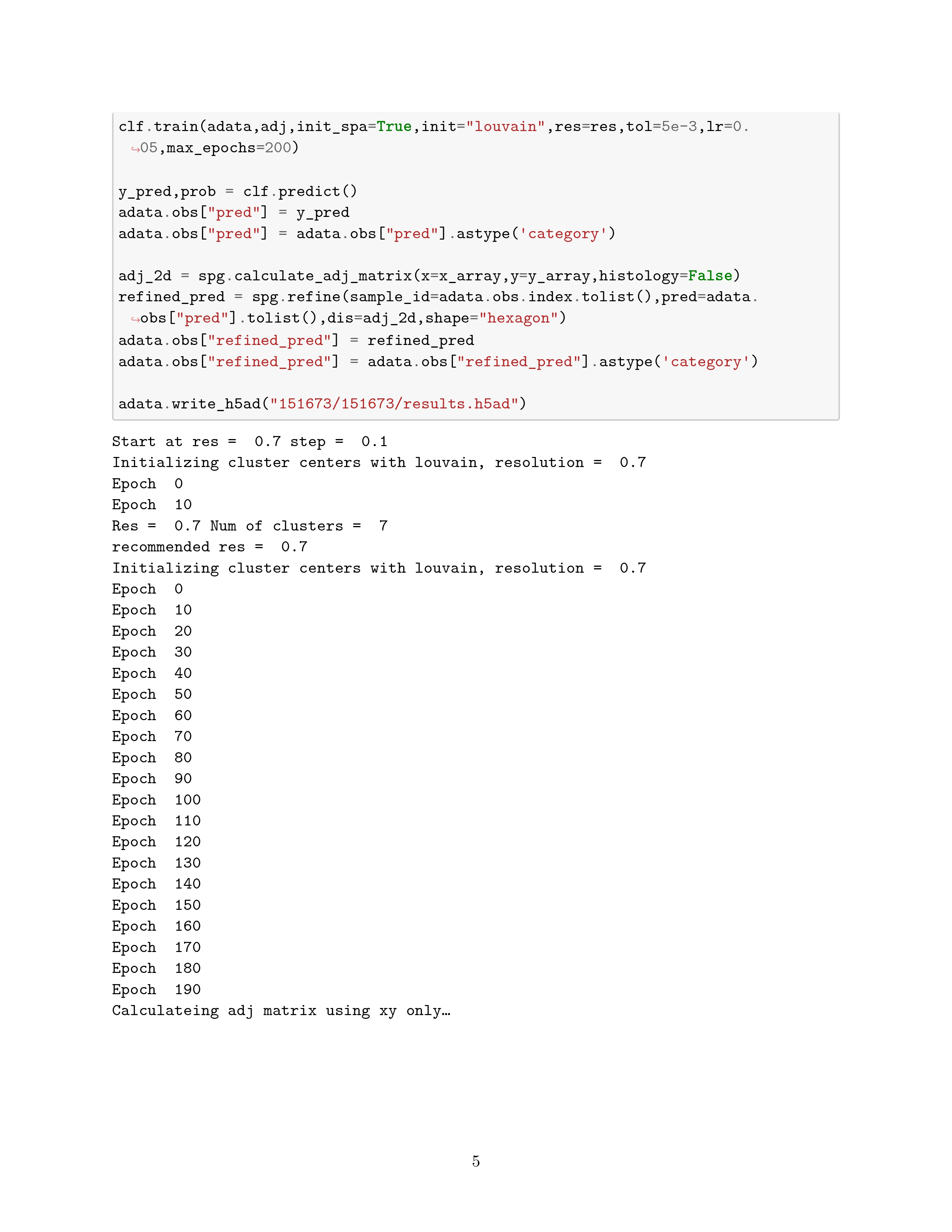
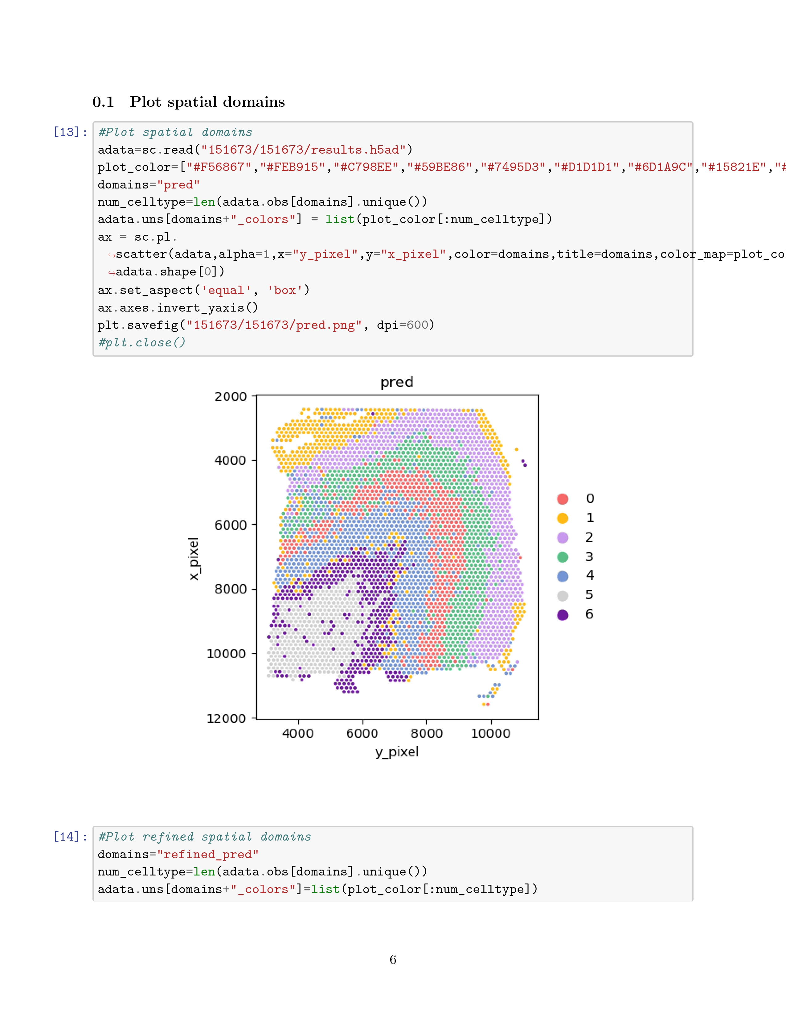
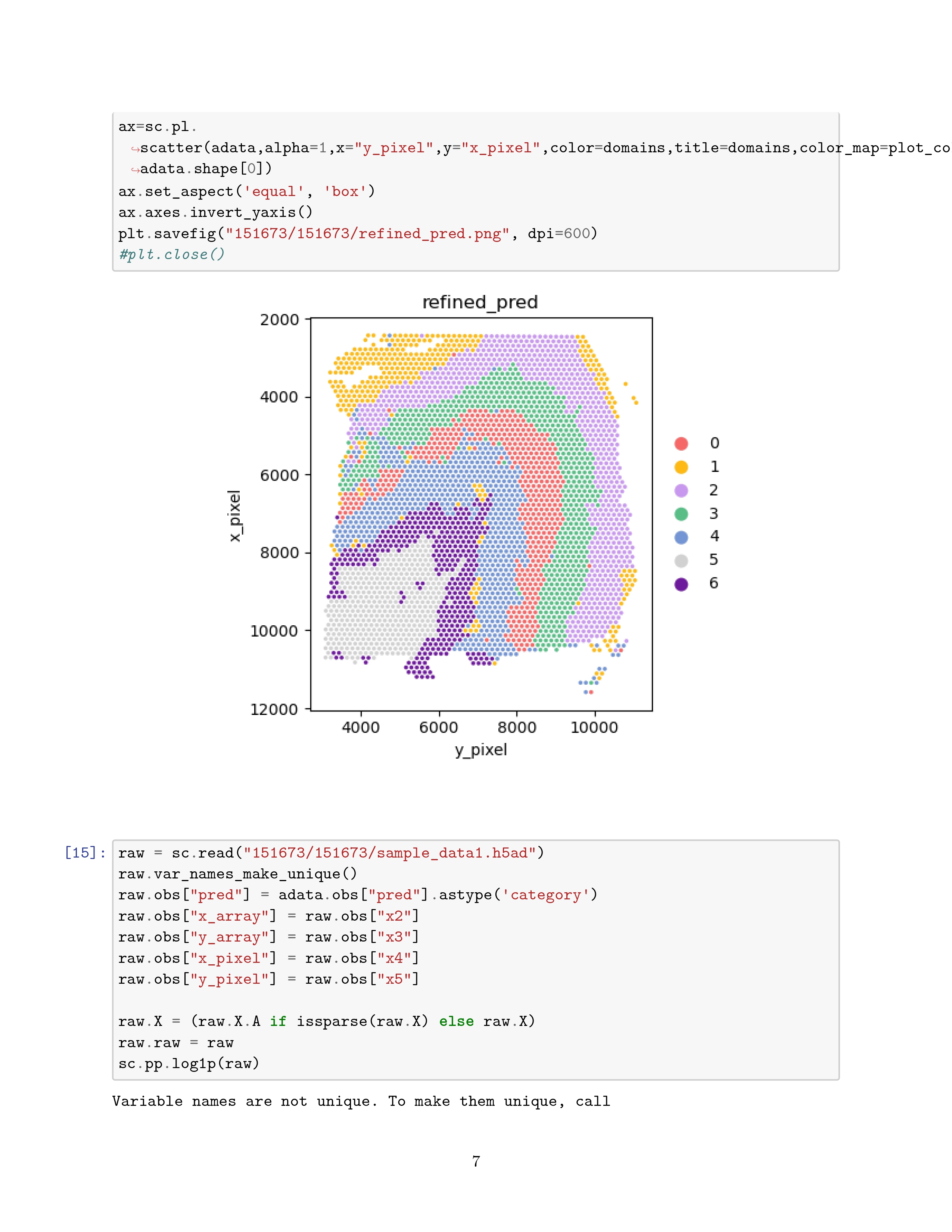
算了，实际上也没遇到什么问题，下面是跑出来的结果

生物学习笔记类算法

# 摘要

# Introduction

# Result

# Overview of SpaGCN and evaluation

# Application to human primary pancreatic (胰腺的) cancer ST data

# 1. P 值（p-value）

# 2. Q 值（q-value）

# 总结对比

# Application to human dorsolateral prefrontal cortex 10x Visium data

# Application to mouse posterior (后面的) brain 10x Visium data

# Application to mouse visual cortex STARmap data

# Discussion

# Methods

# Data prepocessing

# Conversion of SRT data into graph-structured data

# Calculation of distance between two vertices

# Calculation of weight for each edge and construction of graph

# Graph convolutional layer

# Spatial domain identification by clustering

# Detection of SVGs

# 1. 数据来源与表示

# 2. 数据预处理

# 3. 差异表达的统计模型

# （1）假设检验

# 检验方法：

# 关键统计量：

# （2）多重检验校正

# 4. 差异基因筛选

# 5. 可视化与结果解释

# （1）火山图（Volcano Plot）

# （2）热图（Heatmap）

# 6. 后续分析

# 1. 应用场景

# 2. 原理

# （1）假设

# （2）步骤

# 3. 示例

# 步骤 1：合并并排序

# 步骤 2：计算秩和

# 步骤 3：计算 UUU 值

# 步骤 4：查表得 p 值

# 4. 优点

# 5. 限制

# Detection of spatially variable meta genes

# Evaluation of SVGs using Moran'sI and Geary's statics

# 代码

# Clustering

# 原理性的东西

# 图卷积层的计算过程

# 具体计算步骤

# 导入必要的模块

# 定义一个简单的图卷积层

# 创建一个简单的数据集

# 创建模型实例并处理数据

# 具体计算过程

# 示例计算

# 计算支持矩阵 support

# 计算输出特征矩阵 output

# 最终结果

# 解释

# 总结

# 1. self 是什么？为什么 self(X, adj) 可以前向传播？

# 2. 为什么 loss 是一个数，却可以调用 loss.backward() ？底层逻辑是什么？

# loss 的值和张量计算图

# backward() 的作用

# 如何支持梯度计算？

# 3. 为什么可以执行 optimizer.step() ？ optimizer 默认操作的是谁？

# optimizer 是如何绑定模型参数的？

# optimizer.step() 的作用

# 4. self.train() 训练了什么？

# 总结

# SVGs

# 原理性的东西

# 实际使用

Matching_Anything_by_Segmenting_Anything

《素食者》：巧克力味的屎

# 步骤 3：计算 $U$ 值

# 计算支持矩阵 `support`

# 计算输出特征矩阵 `output`

# 1. `self` 是什么？为什么 `self(X, adj)` 可以前向传播？

# 2. 为什么 `loss` 是一个数，却可以调用 `loss.backward()` ？底层逻辑是什么？

# `loss` 的值和张量计算图

# `backward()` 的作用

# 3. 为什么可以执行 `optimizer.step()` ？ `optimizer` 默认操作的是谁？

# `optimizer` 是如何绑定模型参数的？

# `optimizer.step()` 的作用

# 4. `self.train()` 训练了什么？