STAGATE: Deciphering spatial domains from spatially resolved transcriptomics with an adaptive graph attention auto-encoder

主要利用了 Graph Attention Network 里面的方法，创建 3D SNN 时假设不同切片同一位置具有连续性减轻了批次效应。

# 摘要

STAGATE: a graph attention auto-encoder framework accurately identify spatial domains by learning low-dimensional latent embeddings via integrating spatial information and gene expression profiles.

STAGATE adopts an attention mechanism to adaptively learn the similarity of neighboring spots, and an optional cell type-aware module through ingrating the pre-clustering of gene expressions.

We validate STAGATE on diverse spatial transcriptomics datasets generated by different platforms with different spatial resolution

STAGATE could substantially improve the identification accuracy of spatial domains, and denoise the data while preserving spatial expression patterns.

STAGATE could be extended to multiple consecutive sections to reduce batch effects between sections and extracting three-dimensional(3D) expression domains from the reconstructed 3D tissue effectively.

# introduction

non-spatial clustering methods:
1.k-means and Louvain algorithm.
- limited to the small number of spotis or the sparsity according to the different resolutions of ST technologies, and clustering results may be discontinuous in the tissue section
2. utilizes the cell type signatures defined by single-cell RNA-seq to deconvolute the spots.
- They are not applicable to ST data at a resolution of cellular or subcellular levels.
- 例如，某些 ST 技术能够以更高的分辨率直接捕获单个细胞甚至亚细胞层面的基因表达信息。在这种情况下，解卷积的方法可能不适用或没有意义，因为数据本身已经具有高分辨率，能够直接提供细胞级别的信息。

介绍了几个现有的方法：

BayesSpace is a Bayesian statistical method that encourages neighboring spots to belong to the same cluster by introducing spatial neighbor structure into the prior/
Giotto identifies spatial domains by implementing a hidden Markov random field(HMRF) model with the spatial neighbor prior.
stLearn defines the morphological distance based on features extracted from a histology image and utilizes such distances as well as spatial neibor structure to smooth gene expressions.
SEDR employs a deep auto-encoder network for learning gene respresentations and uses a variational graph auto-encoder to simultaneously embed spatial information.
SpaGCN also applies the graph convolutional network to integrate gene expression and spatial location, and further coupled with a self supervised module to identify domains.
RESEPT leverages the supervised image segmentation method to perform tissue structure identification.

STAGATE 全称：Spatially resolved Transcriptomics with an Adaptive Graph ATtention auto-Encoder

# Results

# Overview of STAGATE

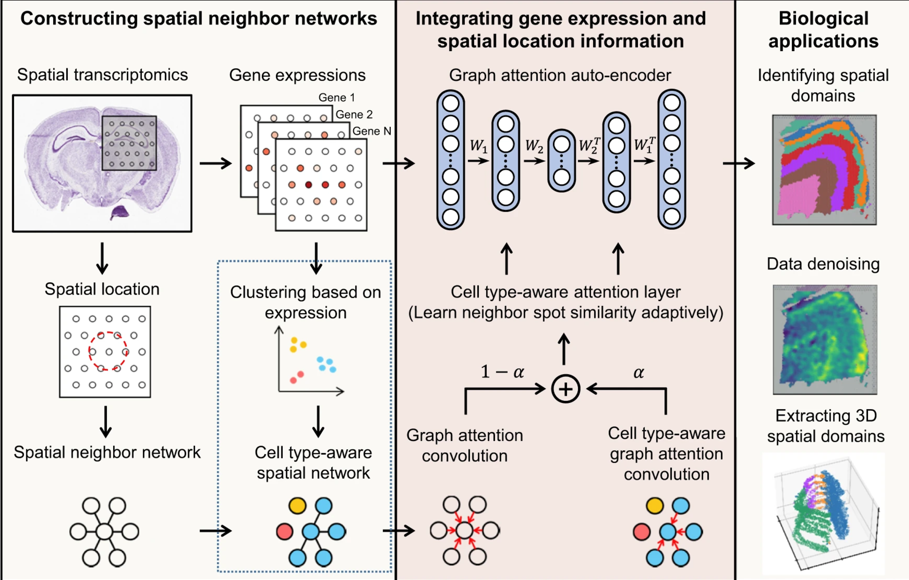
图上面的流程解释的比文字清楚

STAGATE with the cell type-aware module could better learn the spatial similarity.

利用 UMAP 来可视化，利用聚类算法如：mclust 和 Louvain

# STAGATE improves the identification of known layers on the human dorsolateral prefrontal cortex

进一步测试了 STAGATE 的鲁棒性，通过利用不同的 hyper-parameters 对比聚类的准确性，发现这个模型对 encoder structure 和 latent dimension 很敏感

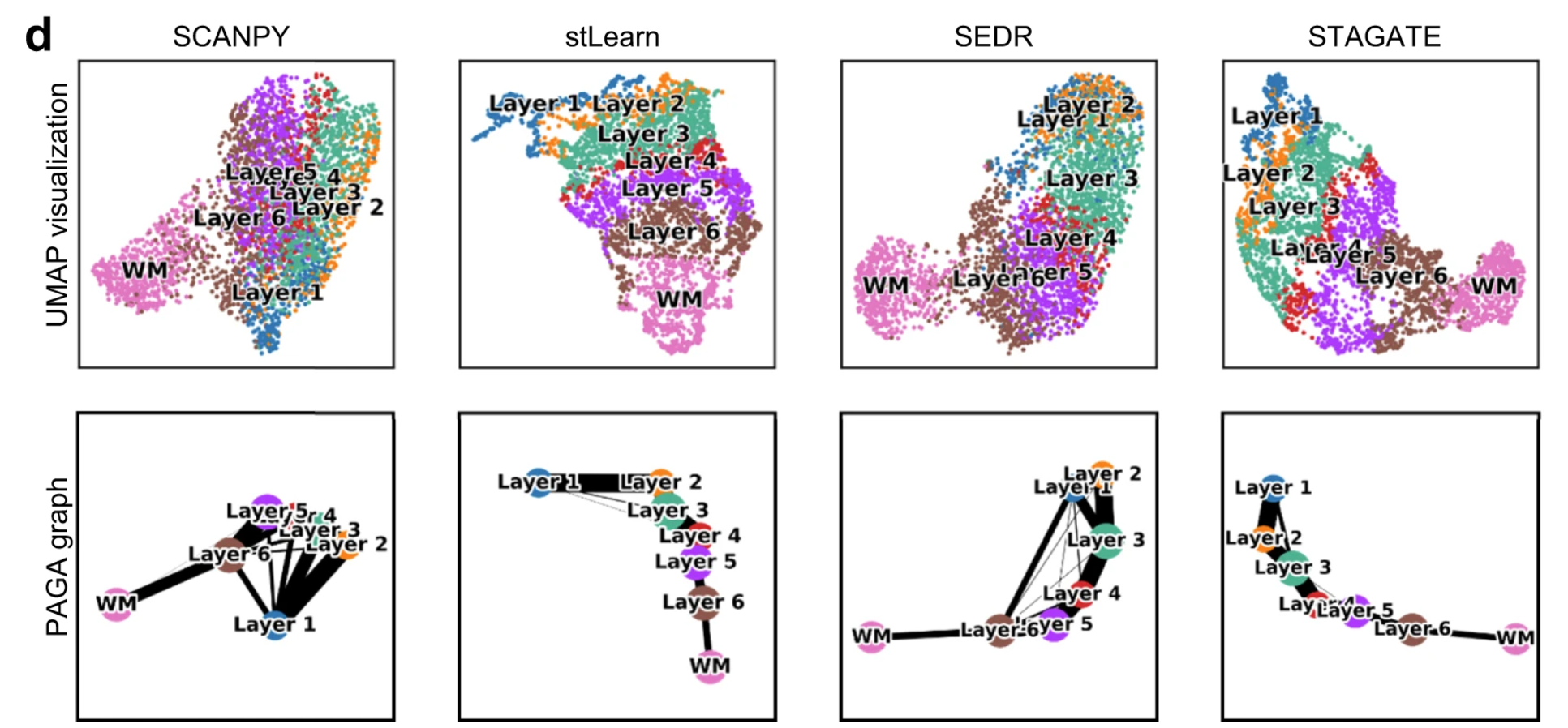
depict the spatial trajectory

# STAGATE enables the identification of tissue structures from ST data of different spatial resolutions.

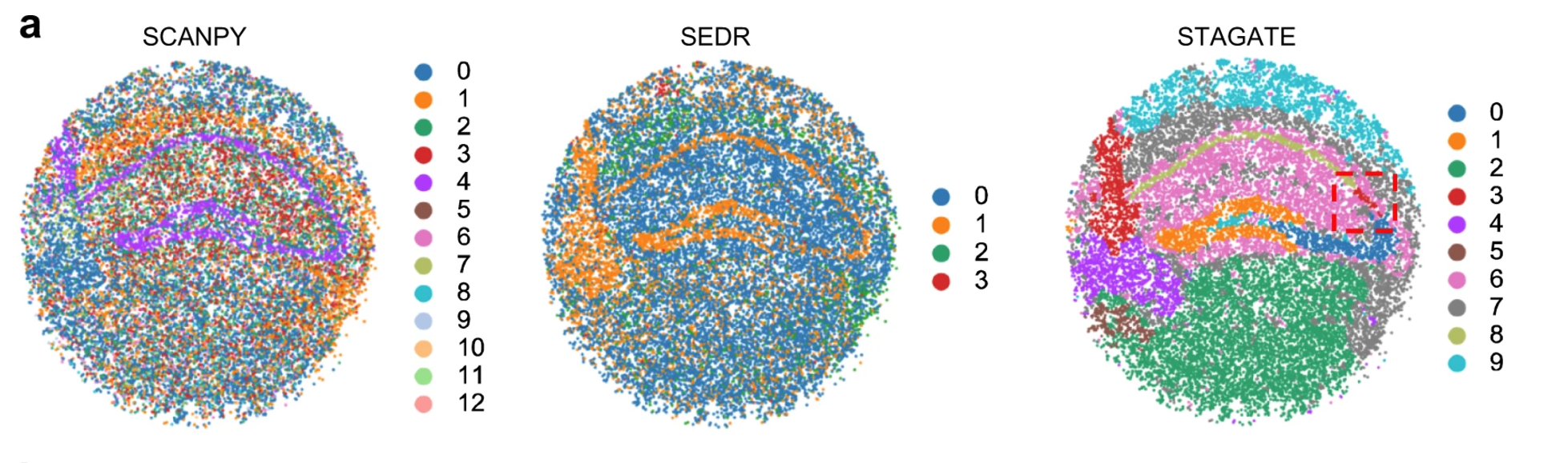
STAGATE can well characterize the tissue structures and uncover the spatial domains, while the clusters identified by SCANPY and SEDR lack clear spatial separation.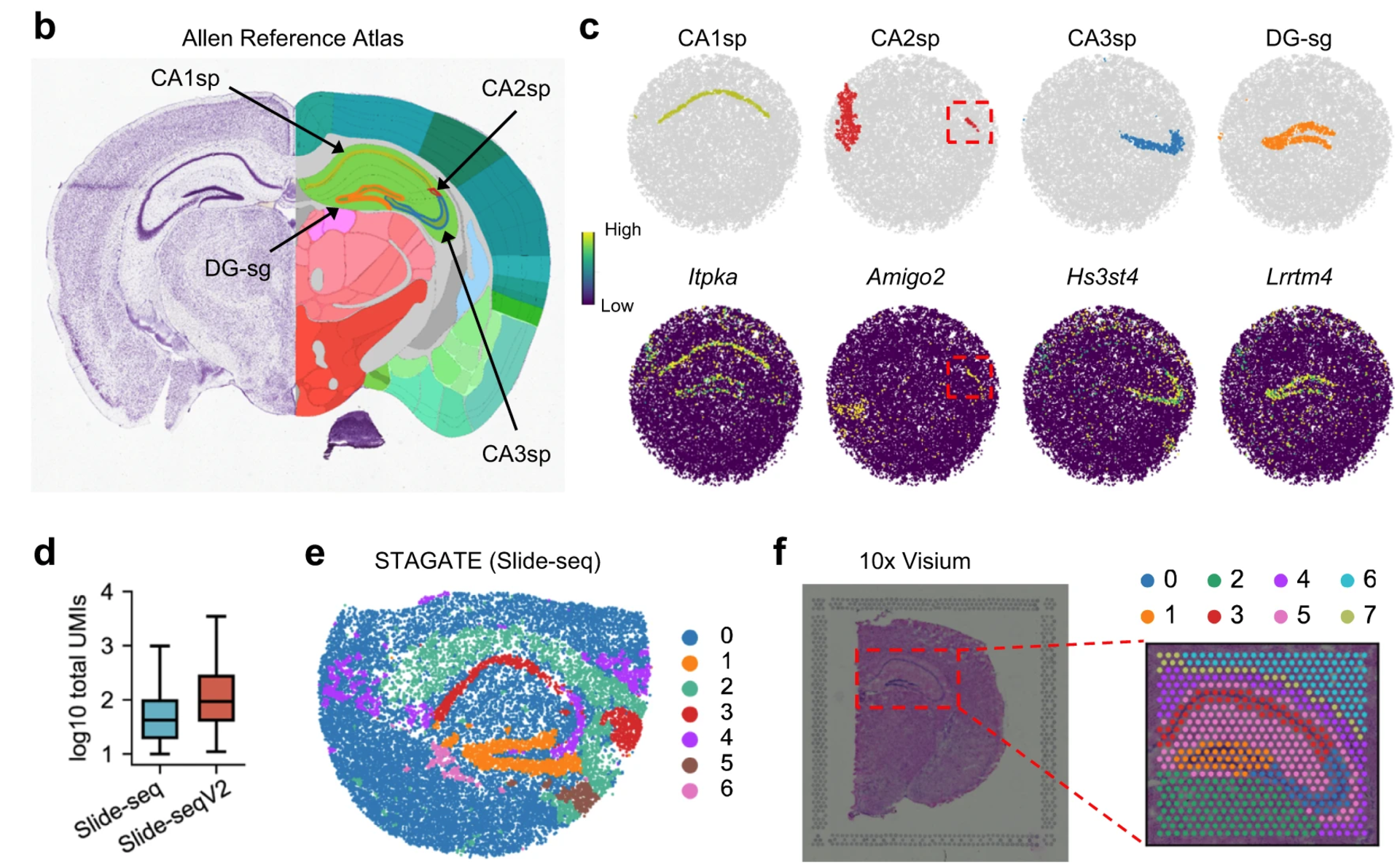

the expressions of many known gene markers also verified the cluster partition of STAGATE.

These results demonstrated that STAGATE can dissect spatial heterogeneity and further uncover spatial expression patterns.

STAGATE depicted the known tissue structures wll except CA2sp on the Slide-seq data(e) and 10x Visium data(f) respectively.

The performance of STAGATE for identifying tissue structures on the mouse olfactory bulb: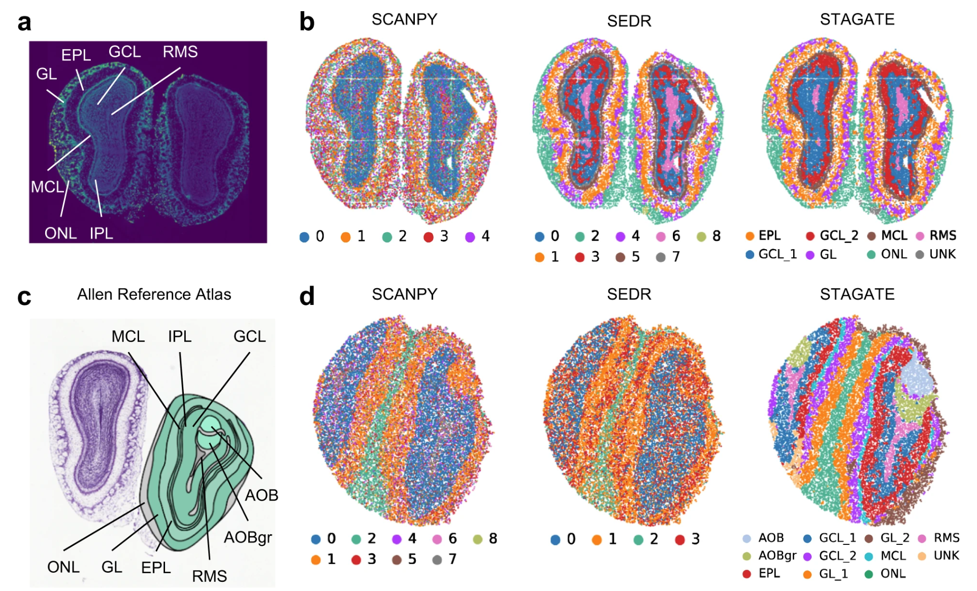

STAGATE recognized the narrow tissue structure MCL clearly, which was validated by the expression of mitral cell marker GABRA1.
Fig b dataset is generated by Stereo-seq
Fig d dataset is generated by Slide-seqV2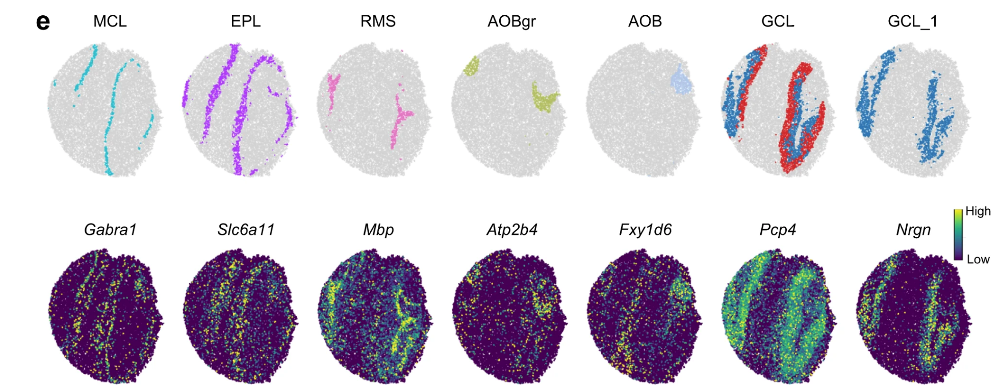

特别的是 STAGATE 检测出了两种先前并未检测出来的空间域：AOB 和 AOBgr
作为佐证，Atp2b4 和 Fxyd6 展现了很强的表达能力。

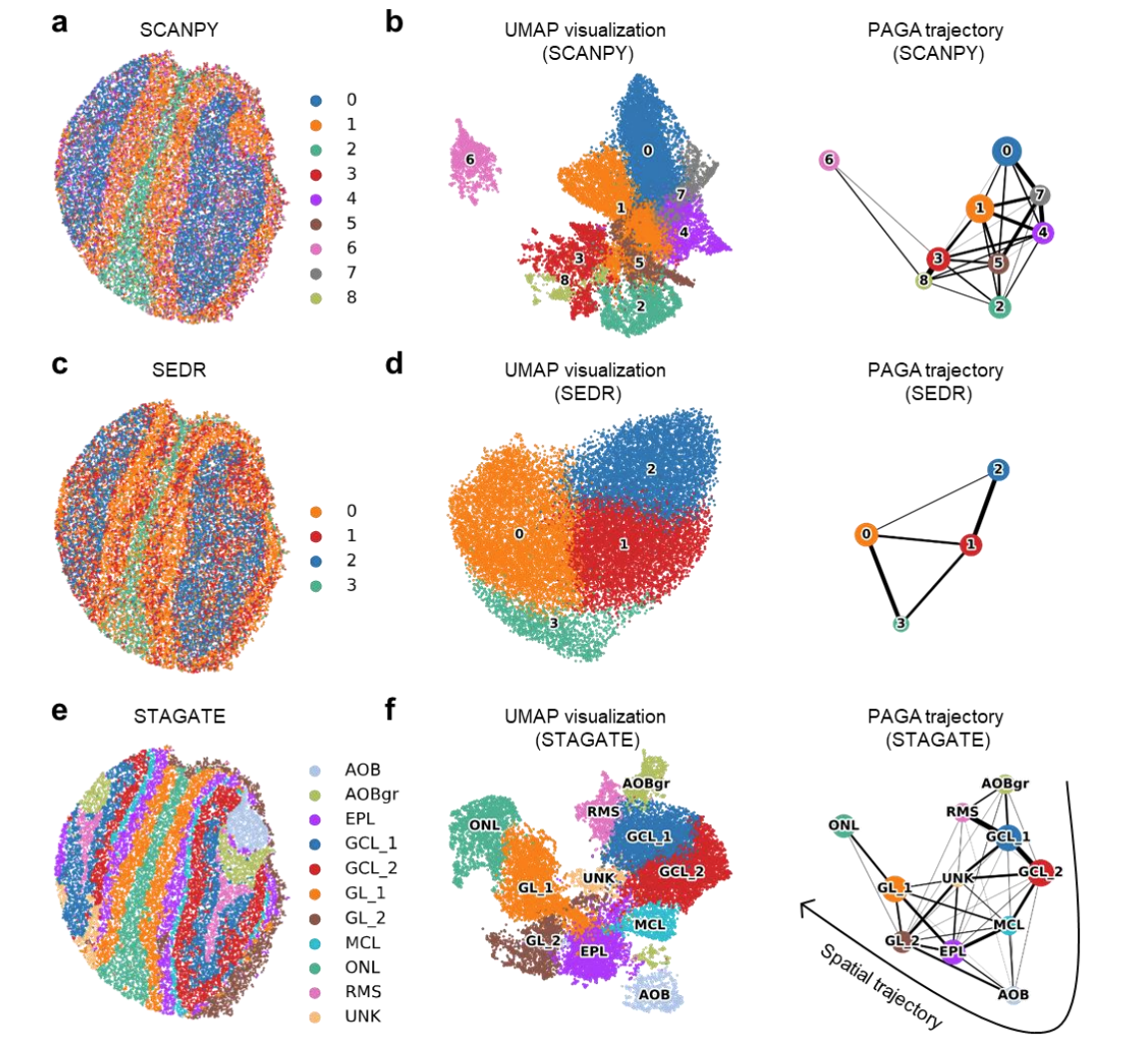
STAGATE delineated the spatial trajectory among the mouse plots as well as the PAGA graphs.

Collectively, these results illustrated the ability of STAGATE to identify tissue structures and reveal their organization from ST data of different spatial resolutions.

# Attention mechanism and cell type-aware module help to better charaterize the similarity between neighboring spots.

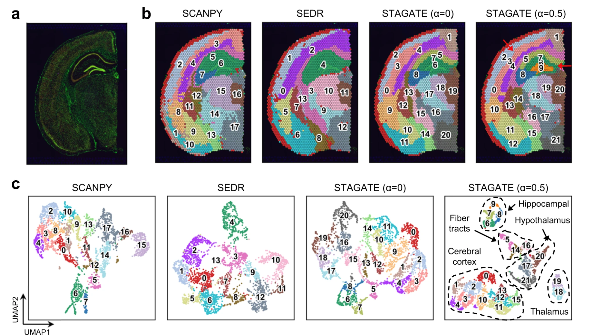
Specifically, in the hippocampal region, STAGATE without the cell type-aware module identified the field CA1(domain7) and CA3(domain8) of Ammon's horn, but did not depict the dentate gyrus structure.

$\alpha=0$ 和 $\alpha=0.5$ 说明了 STAGATE 是否使用了 cell type-aware module.

在 c 图中也能发现，使用了 cell type-aware 模块的 STAGATE 对于 UMAP plot 的操作，更进一步分割了组织结构

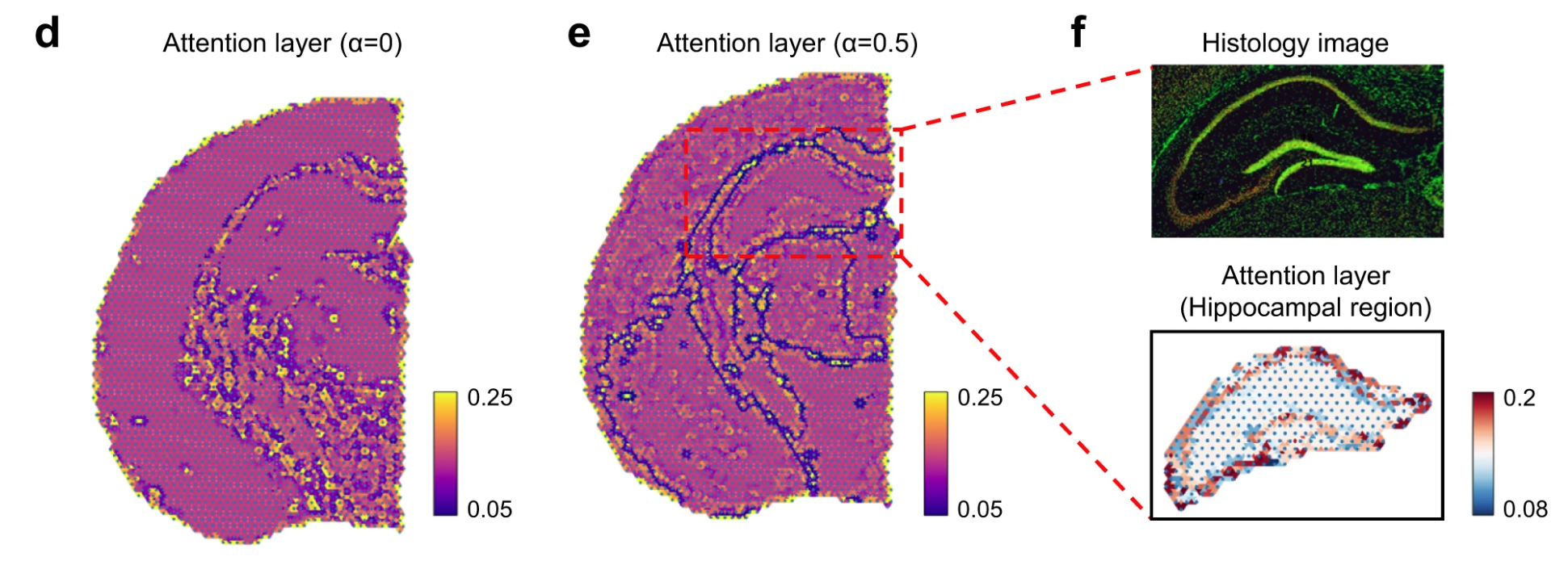
Combining the attention mechanism and the cell type-aware module enhanced the delineation of structure boundaries, and further revealed the spatial similarity within small spatial domains.

Collectively, these results indicated the importance of the attention mechanism and the cell type-aware module for defpicting the similarity between neighboring spots.

# STAGATE denoises gene expressions for better characterizing spatial expression patterns.

STAGATE could denoise and impute gene expressiong.

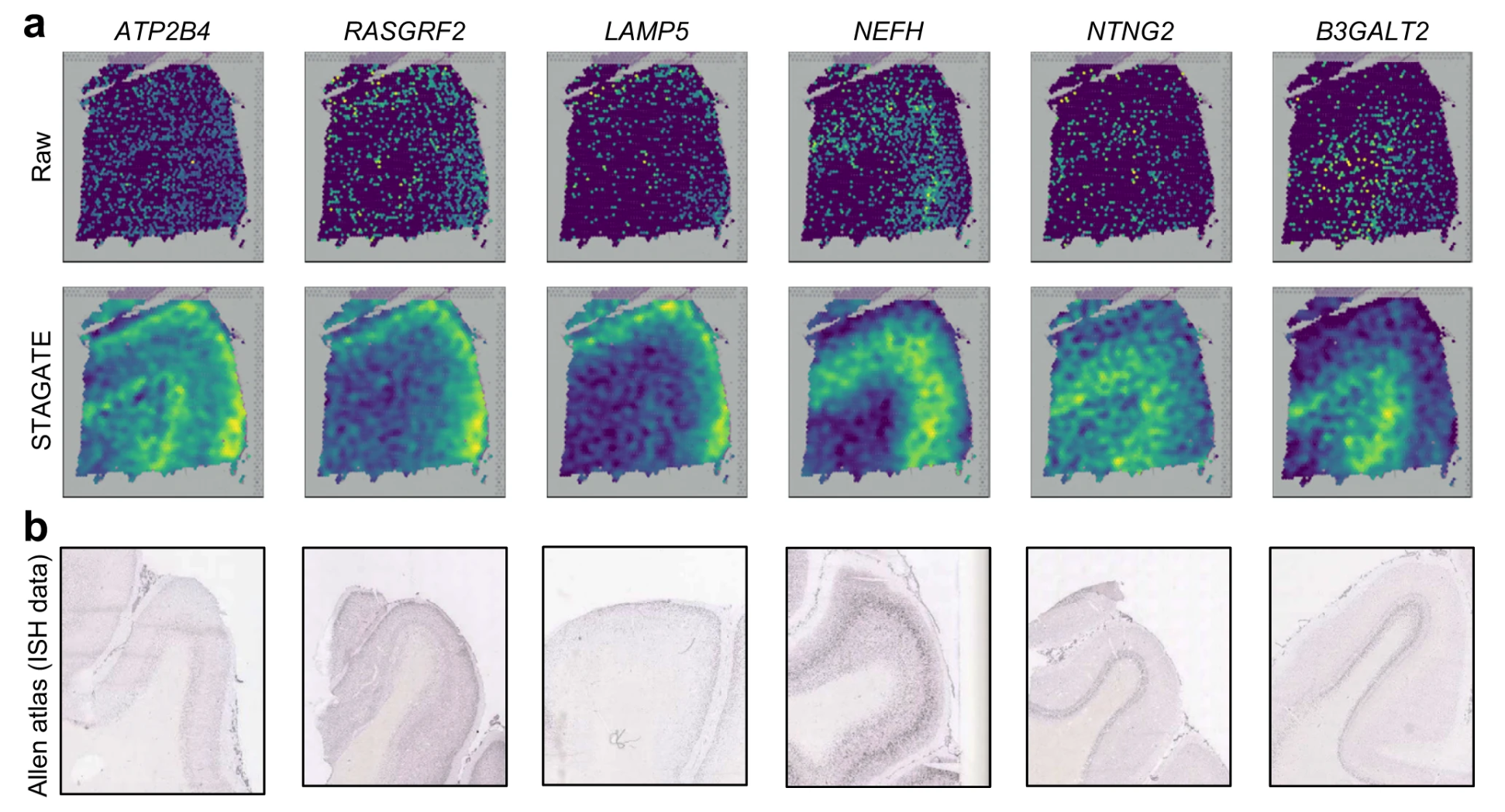
the denoised ones by STAGATE exhibited the laminar enrichment of these layer-marker genes clearly. For example, after denoising, the ATP2B4 gene showed differential expressions in layer 2 and 6, which is consistent with previously reported results, while its raw spatial expression is completely messy.

b 图表示了这些基因通过 in situ hybridization 的方法得到的图像，其实也就是通过染色判断这些基因的位置。

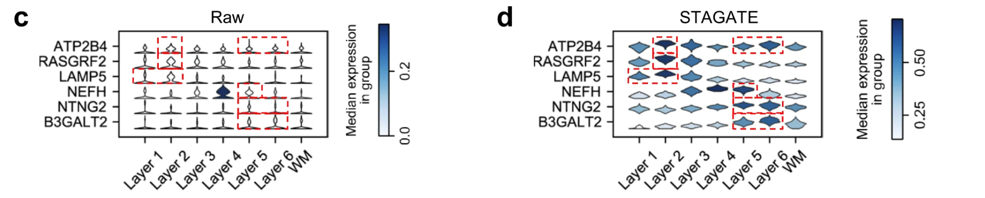
Violin plots 是一种数据可视化工具，结合了 箱线图（box plot） 和 核密度估计图（kernel density plot） 的优点，用来展示数据的分布特性和统计信息。它们通常用于比较多个组的分布情况。

# Violin Plot 的结构

核密度图（Density Plot）：
- Violin plot 的主要部分是左右对称的密度曲线，表示数据分布的概率密度。
- 宽度反映了该值区域的数据密度 —— 越宽表示数据点越集中，越窄表示数据稀疏。
中轴和统计信息：
- Violin plot 的中间可能有类似箱线图的组件：
  - 中位数：通常用一条线标出。
  - 四分位范围（IQR）：即数据的 25% 和 75% 分位点，可能用矩形或线段表示。
  - 异常值：可能用点表示（视具体绘图工具而定）。
对称性：
- Violin plot 通常是左右对称的，但在某些特殊情况下，也可以单边绘制。

# Violin Plot 的用途

分布比较：适用于多个组数据的分布比较，比箱线图更清晰地显示数据的形状（如是否偏态、双峰分布）。
异常值检测：可以观察分布中是否存在异常值或稀疏区域。
多组数据对比：适合分析多组数据在同一变量上的差异。

# Violin Plot 与其他图的区别

特性	Violin Plot	Box Plot	Histogram / 密度图
显示数据分布形状	是	部分	是
统计信息	中位数、四分位数等	中位数、四分位数、异常值	不包含
多组数据比较	是	是	较难
数据密度信息	明确（通过宽度）	不包含	是

Collectively, these results demonstrated the ability of STAGATE to reduce noises and enhance spatial expression patterns.

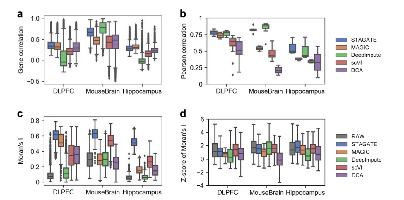
showedits superior in both imputation efficiency and preservation of spatial expression patterns.

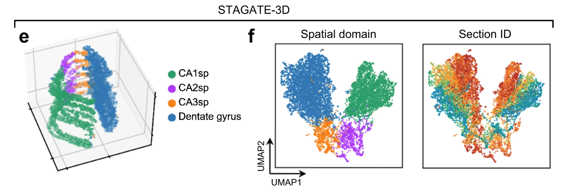
# The usage of 3D SNN leads to better extrction of 3D sptial patterns

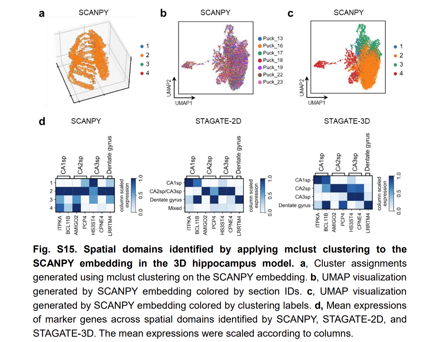
由于数据的稀疏性，SCANPY 的聚类结果是混合的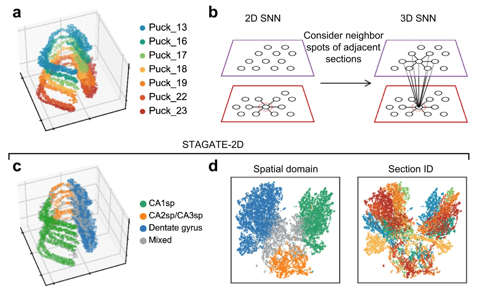

由于批次效应，STAGATE 未能成功识别出 CA2sp 区域

These results illustrated that STAGATE could help to reconstruct 3D tissue models and accurately extract 3D expression patterns by incorporating 3D spatial information.

# Discussion

说明了一些杂七杂八的问题

对前文工作的总结
没有加入 histological image features
对于 single-cell resolution 数据的检测仍然有优越性
STAGATE performs better for ST data of cellular or subcellular resolutions due to the high similarity between neighboring spots
A potential limitation of STAGATE is that it trears neighboring spots from one section the same as those belonging to different sections.
虽然目前在时间方面仍然有优越性，但是终将陷入瓶颈，未来的目标是通过子图的训练策略提升 STAGATE 的可扩展性
STAGATE enables the detection of spatially variable genes within spatial domains.

# Methods

# Construction of SNN

我们预先定义一个半径 $r$
Let $\textbf{A}$ be the adjacency matrix of the SNN, then $\textbf{A}_{ij}$ if and only if the Euclidean distance between spot $i$ and spot $j$ is less than $r$
对于 10x visium data, 我们直接选择最近的 6 个邻居，对于其它的数据，我们根据经验选择 $r$ ，让这个范围内包括 6-15 个邻居。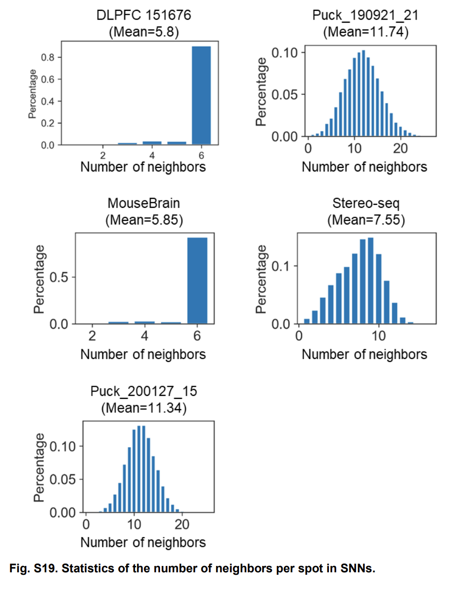

# Construction of cell type-aware SNN(optional)

Specifically, the pre-clustering of gene expressions is conducted by the Louvain algorithm with a small resolution value (set as 0.2 by default) on the PCA embeddings, and STAGATE prunes the edge if the spots of it belong to different clusters.

do not recommend using it to technologies at a resolution of cellular or subcellular levels.Because in this scenario, the similarity between adjacent sites is relatively homogeneous.
而且 technical 本身的噪音也容易被引入。

Encoder:

\begin{equation} \textbf{h}_i^{(k)} = \sigma(\sum_{j\in{S_i}}\textbf{att}_{ij}^{(k)}(\textbf{W}_k\textbf{h}_j^{(k-1)})). \end{equation}

$x_i=h_i^{(0)}$ 其中 $x_i$ 是标准化后的 spot $i$ 的的表达值（应该是基因表达值）， $L$ 是 encoder 层的数量， $k$ 代表第几层。 $\textbf{W}$ 是可训练的权重矩阵。 $\textbf{att}$ is the edge weight between spot $i$ and spot $j$ in the output of the $k$ -th garph attention layer

第 L 层的 encoder layer：

\begin{equation} \textbf{h}_i^{(L)} = \sigma(\textbf{W}_L\textbf{h}_i^{(L-1)}). \end{equation}

Decoder:

\begin{equation} \hat{\textbf{h}_i}^{(k)} = \sigma(\sum_{j\in{S_i}}\hat{\textbf{att}_{ij}}^{(k)}(\hat{\textbf{W}_k}\hat{\textbf{h}_j}^{(k-1)})). \end{equation}

其中 $\hat{\textbf{h}}_i^{(L)} = \textbf{h}_i^{(L)}$
最后一层 decoder：

\begin{equation} \hat{\textbf{h}_i}^{(0)} = \sigma(\hat{\textbf{W}_1}\hat{\textbf{h}_i}^{(1)}). \end{equation}

To avoid overfitting, STAGATE sets $\hat{\textbf{W}}^{(k)} = \textbf{W}^{(k)^T}$ and $\hat{\textbf{att}}^{(k)} = \textbf{att}^{(k)}$ respectively.

att 不是转置其实是因为它本身就是对称的

在 Graph Attention Auto-Encoder (GATE) 的设计中，对于解码器参数设置 $\hat{\textbf{W}}^{(k)} = \textbf{W}^{(k)^T}$ 和 $\hat{\textbf{att}}^{(k)} = \textbf{att}^{(k)}$ ，这是为了避免过拟合并简化模型的参数学习过程。具体原因如下：

# 1. 参数共享减少了模型的自由度

通过设置 $\hat{\textbf{W}}^{(k)} = \textbf{W}^{(k)^T}$ 和 $\hat{\textbf{att}}^{(k)} = \textbf{att}^{(k)}$ ，解码器的权重不再单独学习，而是与编码器的权重共享。这样可以：

减少模型参数数量：减小需要学习的参数规模，降低了模型复杂度，从而减少了过拟合的风险。
强制正则化：通过共享权重，模型在编码和解码时被约束为一种对称映射，提高了泛化能力。

# 2. 对称性假设

对称的邻接信息重构：在图数据中，邻接信息通常是对称的。共享参数可以更好地适应图结构的这一特性。
对偶性设计：编码器将原始图嵌入到一个潜在空间，解码器再将该潜在空间的表示恢复为原始空间。权重共享实际上保证了解码器对编码器的 “反演” 能力。

# 3. 理论支持

将解码器权重设为编码器权重的转置，在数学上等价于假设潜在表示空间的映射是线性可逆的：

\begin{equation} \textbf{Z} = f(\textbf{X}, \textbf{A}; \textbf{W}, \textbf{att}), \hat{\textbf{A}} = g(\textbf{Z}; \hat{\textbf{W}}, \hat{\textbf{att}}), \end{equation}

其中 $g$ 是解码器。如果 $g$ 的参数由 $f$ 的参数直接确定，模型更倾向于在权重共享的限制下寻找稳定的表示。

# 4. 实践效果

在实际操作中，权重共享可以显著提升训练效率和模型性能：

避免了过拟合引起的解码器参数冗余。
保持了训练的稳定性，尤其是在小数据集或稀疏图上表现明显。

# 5. STAGATE 的特殊性

在 STAGATE 中（针对空间转录组学），数据通常具有显著的稀疏性和局部性。权重共享在这种高噪声数据下尤为重要，因为它降低了解码器单独学习复杂模式的风险，确保模型专注于全局结构和局部关联的核心信息。

Graph attention layer:

\begin{equation} e_{ij}^k = Sigmoid(\textbf{v}_s^{(K)^T}(\textbf{W}_k\textbf{h}_i^{(k-1)})+\textbf{v}_r^{(K)^T}(\textbf{W}_k\textbf{h}_j^{(k-1)})). \end{equation}

$\textbf{v}_s^{(K)}$ and $\textbf{v}_r^{(K)}$ are the trainable weight vectors and Sigmoid represents the sigmoid activation function.

下面是标准化：

\begin{equation} att_{ij}^{(k)} = \frac{exp(e_{ij}^{(k)})}{\sum\limits_{i\in\Upsilon_i}exp(e_{ij}^{(k)})}. \end{equation}

cell type-aware 模块的使用：

\begin{equation} \textbf{att}_{ij} = (1-\alpha)\textbf{att}_{ij}^{spatial}+\alpha\textbf{att}_{ij}^{aware}. \end{equation}

损失函数：

\begin{equation} \sum\limits^{N}_{i=1}\| x_i-\hat{h}_i^0\|_2. \end{equation}

# Identifying differential expressed genes

Benjamin-Hochberg 调整（Benjamini-Hochberg Adjustment，简称 BH 调整）是一种用于多重假设检验的统计方法，旨在控制假发现率（False Discovery Rate, FDR）。FDR 是指被拒绝的零假设中实际为真假设的比例。

在进行多重假设检验时，由于同时进行多个检验，直接使用原始的 $p$ - 值会导致较高的错误发现概率（如大量的第一类错误）。BH 调整通过对 $p$ - 值进行排序和阈值校正，来控制 FDR，使研究者能在多个检验中更有信心地拒绝零假设。

# 算法步骤

假设我们有 $m$ 个假设检验，计算得到对应的 $p$ - 值为 $p_1, p_2, \ldots, p_m$ ：

排序 $p$ - 值：
- 对 $p$ - 值进行升序排序，得到排序后的 $p$ - 值 $p_{(1)} \leq p_{(2)} \leq \cdots \leq p_{(m)}$ ，对应的原始假设分别为 $H_{(1)}, H_{(2)}, \ldots, H_{(m)}$ 。
设定目标 FDR：
- 选择一个目标 FDR，记为 $q$ （通常是 0.05 或 0.10）。
计算调整后的阈值：
- 对每个排序后的 $p$ - 值计算阈值：\begin{equation} p_{\text{threshold}, (i)} = \frac{i}{m} q \end{equation} 其中 $i$ 是排序中 $p_{(i)}$ 的位置， $m$ 是假设检验总数。
确定显著性水平：
- 找到最大的 $k$ 使得：\begin{equation} p_{(k)} \leq p_{\text{threshold}, (k)} \end{equation}
- 记 $H_{(1)}, H_{(2)}, \ldots, H_{(k)}$ 为显著假设，即可拒绝对应的零假设。
调整 $p$ - 值（可选）：
- 计算调整后的 $p$ - 值，用于更直观地评估显著性：\begin{equation} p'_{(i)} = \min\left( \frac{m}{i} p_{(i)}, 1 \right) \end{equation}

# 核心思想

BH 调整通过动态的 $p$ - 值阈值来控制 FDR，使得拒绝的假设数量尽量多，但整体错误率保持在目标范围内。
相比更严格的 Bonferroni 校正，BH 调整更宽松，因此在实际应用中拒绝的假设通常更多，但仍然具有较高的置信度。

# 适用场景

基因组学和多组学数据分析：
- 例如 RNA-seq 或微阵列数据分析中，往往需要同时对成千上万的基因表达水平进行显著性检验。
机器学习和深度学习：
- 当对多个特征或模型进行假设检验时，BH 调整可用于选择显著性特征或结果。
临床研究：
- 当研究多个治疗变量或药物反应的显著性时，BH 调整有助于减少假发现的风险。

# 与其他方法的比较

Bonferroni 校正：
- 控制的是整体第一类错误率（FWER）。
- 更严格，显著性检测结果通常较少。
- 适用于较少假设检验。
Benjamini-Hochberg 校正：
- 控制的是假发现率（FDR）。
- 更宽松，显著性检测结果更多。
- 适用于大量假设检验。

# 示例

假设有 5 个假设检验，得到的 $p$ - 值为：$$\begin {equation} 0.01, 0.03, 0.05, 0.10, 0.20 \end {equation}$$，设目标 FDR $q = 0.10$ ：

排序 $p$ - 值：$$\begin {equation} 0.01, 0.03, 0.05, 0.10, 0.20 \end {equation}$$
计算阈值：$$\begin {equation} \frac {1}{5} \cdot 0.10, \frac {2}{5} \cdot 0.10, \frac {3}{5} \cdot 0.10, \frac {4}{5} \cdot 0.10, \frac {5}{5} \cdot 0.10 \end {equation}$$，即 $$\begin {equation} 0.02, 0.04, 0.06, 0.08, 0.10 \end {equation}$$
找到最大 $k$ 使 $p_{(k)} \leq p_{\text{threshold}, (k)}$ ：只有 $p_{(1)} = 0.01$ 和 $p_{(2)} = 0.03$ 满足条件，因此拒绝对应的 2 个假设。

# 结论

BH 调整是一种平衡严格性和敏感性的校正方法，尤其适合大规模多重检验问题。

# Identification of 3D spatial domains using STAGATE

the batch effect between sections hinders the extraction of 3D spatial patterns. Here we introduced a 3D SNN by incorporating the 2D SNN of each section and the SNN between adjacent sections to alleviate the batch effect between consecutive sections.

The key idea of the usage of 3D SNN is that the biological differences between consecutive sections should be continuous, so we can enhance the similarity between adjacent sections to eliminate the discontinuous independent technical noises.

# 代码

安装 pyG 时遇到 torch-sparse 报错：

在这个网站上找对应的版本

照搬代码也没意思，就记录一下自己觉得有价值、可以学习的地方吧。

这里面的方法其实主体是 Graph Attention Network，然后在此基础上进行操作。看来是有必要去阅读一下这篇论文，毕竟也不是主要工作，近期去泛读一下吧，就下篇文章先看这个再去看 MENDER 那篇文章。

参数和方法：

\begin{equation} \mathbf{x}^{\prime}_i = \alpha_{i,i}\mathbf{\Theta}\mathbf{x}_{i} + \sum_{j \in \mathcal{N}(i)} \alpha_{i,j}\mathbf{\Theta}\mathbf{x}_{j}, \end{equation}

where the attention coefficients $\alpha_{i,j}$ are computed as

\begin{equation} \alpha_{i,j} = \frac{ \exp\left(\mathrm{LeakyReLU}\left(\mathbf{a}^{\top} [\mathbf{\Theta}\mathbf{x}_i \, \Vert \, \mathbf{\Theta}\mathbf{x}_j] \right)\right)} {\sum_{k \in \mathcal{N}(i) \cup \{ i \}} \exp\left(\mathrm{LeakyReLU}\left(\mathbf{a}^{\top} [\mathbf{\Theta}\mathbf{x}_i \, \Vert \, \mathbf{\Theta}\mathbf{x}_k] \right)\right)}. \end{equation}

Args:

in_channels (int or tuple): Size of each input sample, or -1 to derive the size from the first input(s) to the forward method. A tuple corresponds to the sizes of source and target dimensionalities.
out_channels (int): Size of each output sample.
heads (int, optional): Number of multi-head-attentions.(default: 1 )
concat (bool, optional): If set to : False , the multi-head
attentions are averaged instead of concatenated.
(default: True )
negative_slope (float, optional): LeakyReLU angle of the negative
slope. (default: 0.2 )
dropout (float, optional): Dropout probability of the normalized
attention coefficients which exposes each node to a stochastically
sampled neighborhood during training. (default: :obj: 0 )
add_self_loops (bool, optional): If set to :obj: False , will not add
self-loops to the input graph. (default: :obj: True )
bias (bool, optional): If set to :obj: False , the layer will not learn
an additive bias. (default: :obj: True )
kwargs (optional): Additional arguments of :class: torch_geometric.nn.conv.MessagePassing .

Dropout 是一种正则化技术，用于神经网络训练过程中，帮助防止模型过拟合（overfitting）。它的核心思想是，在每次训练迭代中，随机地将一些神经元的输出值置为零，从而削弱神经元间的依赖性，提高模型的泛化能力

nn.init.xavier_normal_ 是 PyTorch 中的一个函数，用于对神经网络层的权重进行初始化。它实现了 Xavier initialization 的一种变体，采用正态分布来初始化权重。其目的是保证神经网络的输入和输出的方差在前向传播和反向传播中尽量保持一致，避免梯度爆炸或消失的问题。

# Xavier Initialization

Xavier 初始化方法来源于论文 "Understanding the difficulty of training deep feedforward neural networks"（Glorot & Bengio, 2010）。它的核心思想是：

初始化权重时的分布方差依赖于输入和输出的神经元个数：\begin{equation} \text{Var}(w) = \frac{2}{\text{fan\_in} + \text{fan\_out}} \end{equation} 其中：
- fan_in 是该层输入的神经元个数。
- fan_out 是该层输出的神经元个数。

Xavier 初始化有两种实现方式：

均匀分布（Xavier Uniform）： 从区间 $[-a, a]$ 中采样， $a = \sqrt{\frac{6}{\text{fan\_in} + \text{fan\_out}}}$ 。
正态分布（Xavier Normal）： 从均值为 0，标准差为 $\sqrt{\frac{2}{\text{fan\_in} + \text{fan\_out}}}$ 的正态分布中采样。

# `nn.init.xavier_normal_` 的工作原理

它基于正态分布来初始化权重。
对于权重张量中的每个值，按照以下公式采样：\begin{equation} w \sim \mathcal{N}\left(0, \sqrt{\frac{2}{\text{fan\_in} + \text{fan\_out}}}\right) \end{equation}

# 函数签名

1	torch.nn.init.xavier_normal_(tensor, gain=1.0)

# 参数

tensor : 要初始化的权重张量。
gain : 一个缩放因子，用于调整初始化分布的标准差。通常用 1（默认值）或非线性激活函数的导数相关值（例如对于 ReLU 激活，可以设置为 $\sqrt{2}$ ）。

# 使用示例

以下示例展示如何使用 nn.init.xavier_normal_ 初始化权重：

import torch
import torch.nn as nn

# 创建一个权重张量
weights = torch.empty(3, 5)  # 假设是一个 3x5 的线性层权重矩阵

# 使用 xavier_normal_ 初始化权重
nn.init.xavier_normal_(weights)
print(weights)

# 在模型中的应用

通常在构造自定义神经网络时，我们可以用 xavier_normal_ 对权重进行初始化。例如：

class MyModel(nn.Module):
    def __init__(self):
        super(MyModel, self).__init__()
        self.fc = nn.Linear(10, 5)  # 全连接层
    
    def reset_parameters(self):
        # 初始化全连接层的权重
        nn.init.xavier_normal_(self.fc.weight)

model = MyModel()
model.reset_parameters()

# Xavier Initialization 的优势

平衡了输入和输出的方差，使得前向传播和反向传播的梯度不会过大或过小。
提高训练的收敛速度和稳定性，尤其是深层网络中。

对于代码：

1	x_src = x_dst = torch.mm(x, self.lin_src).view(-1, H, C)

其中 H 和 C 代表

1	H, C = self.heads, self.out_channels

$\mathbf{x}\to\mathbf{\Theta}\mathbf{x}\to heads, out\_channels$

# 拆解解析：

torch.mm(x, self.lin_src)
- 功能：矩阵乘法。对输入特征 x 应用权重矩阵 self.lin_src ，完成线性变换。
- 参数：
  - x 是输入节点的特征矩阵，形状为 $(N, F_{\text{in}})$ $(N, F_{in})$ ，其中：
    - $N$ 是节点的数量。
    - $F_{\text{in}}$ 是每个节点的输入特征维度。
  - self.lin_src 是权重矩阵，形状为 $(F_{\text{in}}, H \cdot C)$ $(F_{in}, H \cdot C)$ ，其中：
    - $H$ 是多头注意力的头数（ heads ）。
    - $C$ 是每个注意力头的输出特征维度。
- 结果：矩阵乘法的输出形状为 $(N, H \cdot C)$ ，即所有节点的特征经过线性变换后的新表示。
.view(-1, H, C)
- 功能：对上述结果重新调整形状，便于后续的多头处理。
- 参数：
  - -1 表示保持第一个维度的大小（即节点数量 $N$ ）。
  - H 表示多头注意力的头数。
  - C 表示每个头的输出特征维度。
- 结果：输出形状变为 $(N, H, C)$ ，即每个节点特征被拆分为 $H$ 个注意力头，每个头有 $C$ 个维度的特征。
x_src = x_dst = ...
- 功能：将线性变换的结果赋值给 x_src 和 x_dst ，分别代表源节点特征和目标节点特征。
- 场景：
  - 在无向图或默认情况下，源节点和目标节点特征是相同的，所以 x_src 和 x_dst 被赋值为同一个结果。
  - 在二部图（bipartite graph）中， x_src 和 x_dst 可以分别代表不同的特征。

# 直观示例：

假设：

输入特征矩阵 x 为：
\begin{equation} x = \begin{bmatrix} 1 & 2 & 3 \\ 4 & 5 & 6 \end{bmatrix}, \quad \text{形状: } (2, 3) \end{equation}
（2 个节点，每个节点有 3 维特征）。
权重矩阵 self.lin_src 为：
\begin{equation} \text{self.lin_src} = \begin{bmatrix} 0.1 & 0.2 & 0.3 & 0.4 \\ 0.5 & 0.6 & 0.7 & 0.8 \\ 0.9 & 1.0 & 1.1 & 1.2 \end{bmatrix}, \quad \text{形状: } (3, 4) \end{equation}
（输入维度 3，输出维度为 $H \cdot C = 4$ ）。

# 计算过程：

矩阵乘法：
\begin{equation} \text{torch.mm}(x, \text{self.lin_src}) = \begin{bmatrix} 1 & 2 & 3 \\ 4 & 5 & 6 \end{bmatrix} \cdot \begin{bmatrix} 0.1 & 0.2 & 0.3 & 0.4 \\ 0.5 & 0.6 & 0.7 & 0.8 \\ 0.9 & 1.0 & 1.1 & 1.2 \end{bmatrix} = \begin{bmatrix} 4.2 & 4.8 & 5.4 & 6.0 \\ 9.9 & 11.4 & 12.9 & 14.4 \end{bmatrix} \end{equation}
输出形状为 $(2, 4)$ 。
调整形状：
假设多头 $H = 2$ ，每头输出特征维度 $C = 2$ 。将形状从 $(2, 4)$ 调整为 $(2, 2, 2)$ ：
\begin{equation} \text{view(-1, H, C)} = \begin{bmatrix} [[4.2, 4.8], [5.4, 6.0]] \\ [[9.9, 11.4], [12.9, 14.4]] \end{bmatrix} \end{equation} 表示每个节点有两个注意力头，每个头有 2 维特征。

# 总结：

torch.mm(x, self.lin_src) 将输入特征与权重矩阵相乘，得到新的特征表示。
.view(-1, H, C) 将结果重塑为 $(N, H, C)$ ，为每个节点的每个注意力头分配特征。
通过 x_src 和 x_dst 分别表示源节点和目标节点的特征，支持二部图和无向图。

alpha.unsqueeze (-1) 的含义

基本功能：
unsqueeze (dim) 是 PyTorch 中用于在指定维度插入一个新轴（维度）的操作。
dim=-1 表示在最后一个维度新增一个轴。

torch_geometric.nn.MessagePassing 是 PyTorch Geometric 中的一个核心基类，用于实现图神经网络（Graph Neural Network, GNN）中的消息传递机制。通过继承这个类，我们可以轻松定义各种基于消息传递的图神经网络模型。

# `MessagePassing` 的核心机制

消息传递的核心思想是在图的边上计算信息，然后聚合到节点上。 MessagePassing 提供了以下主要的流程：

消息传递（ message ）：计算边的特征或从相邻节点收集的信息。
消息聚合（ aggregate ）：将邻居节点的信息聚合到中心节点上。
更新（ update ）：用聚合后的信息更新节点特征。
传播（ propagate ）：协调消息传递流程，调用 message 、 aggregate 和 update 方法。

# `MessagePassing` 的核心方法

# 1. 初始化： `init`

MessagePassing 类初始化时可以通过 aggr 参数指定聚合方式：

"add" ：加和邻居消息（默认）。
"mean" ：求平均。
"max" ：取最大值。

from torch_geometric.nn import MessagePassing

class MyGNN(MessagePassing):
    def __init__(self):
        super().__init__(aggr='mean')  # 聚合方式为求平均

# 2. 消息传播： `propagate`

propagate 是消息传递的入口。它需要以下关键参数：

edge_index ：边的索引。
x ：节点特征。
可选参数：如 edge_weight （边的权重）。

propagate 会调用 message 、 aggregate 和 update 。

1
2
3

class MyGNN(MessagePassing):
    def forward(self, x, edge_index):
        return self.propagate(edge_index, x=x)  # 触发消息传递流程

# 3. 消息生成： `message`

message 定义了如何生成消息，通常依赖边两端的特征（ x_i 和 x_j ），以及边的属性（如果有）。

x_i ：目标节点的特征（中心节点）。
x_j ：源节点的特征（邻居节点）。
edge_attr （可选）：边的属性。

1
2
3

class MyGNN(MessagePassing):
    def message(self, x_j):
        return x_j  # 示例：直接返回邻居节点特征

# 4. 消息聚合： `aggregate`

aggregate 定义了如何对接收到的消息进行聚合，通常使用的是初始化时指定的聚合方式。如果需要自定义，可以覆盖该方法。

1
2
3

class MyGNN(MessagePassing):
    def aggregate(self, inputs, index):
        return torch.mean(inputs, dim=0)  # 示例：对所有邻居求平均

# 5. 更新： `update`

update 定义了如何使用聚合后的特征更新节点特征。

1
2
3

class MyGNN(MessagePassing):
    def update(self, inputs):
        return inputs  # 示例：直接返回聚合后的特征

# 完整示例：自定义 GCN

以下是实现一个简单图卷积网络（Graph Convolutional Network, GCN）的示例：

import torch
from torch_geometric.nn import MessagePassing
from torch_geometric.utils import add_self_loops, degree

class GCNConv(MessagePassing):
    def __init__(self, in_channels, out_channels):
        super().__init__(aggr='add')  # 使用加和作为聚合方式
        self.linear = torch.nn.Linear(in_channels, out_channels)

    def forward(self, x, edge_index):
        # 添加自环
        edge_index, _ = add_self_loops(edge_index, num_nodes=x.size(0))

        # 计算节点的度
        row, col = edge_index
        deg = degree(col, x.size(0), dtype=x.dtype)
        deg_inv_sqrt = deg.pow(-0.5)
        deg_inv_sqrt[deg_inv_sqrt == float('inf')] = 0

        # 计算归一化因子
        norm = deg_inv_sqrt[row] * deg_inv_sqrt[col]

        # 调用 propagate 进行消息传递
        return self.propagate(edge_index, x=x, norm=norm)

    def message(self, x_j, norm):
        # 消息为归一化的特征
        return norm.view(-1, 1) * x_j

    def update(self, aggr_out):
        # 更新后的节点特征
        return self.linear(aggr_out)

# 测试
x = torch.rand(4, 16)  # 4 个节点，每个节点 16 维特征
edge_index = torch.tensor([[0, 1, 2, 3], [1, 0, 3, 2]])  # 边的索引

conv = GCNConv(16, 32)  # 输入 16 维，输出 32 维
out = conv(x, edge_index)
print(out.shape)  # 输出: torch.Size([4, 32])

# 常见用法

GCN: 使用加权和的消息传递。
GAT: 在 message 方法中引入注意力机制。
GraphSAGE: 在 aggregate 方法中自定义聚合方式（如均值或池化）。

通过继承 MessagePassing ，可以高度灵活地实现各种图神经网络模型，同时复用其高效的计算框架和操作优化。

学到现在，我认为这个对细胞数据进行聚类的思想就是把相似的区域聚类在一起，不同的区域分开，主要的思想方法就是加强数据的隐藏信息，只不过每种方法采用的方式不同。最关键的一点就是利用邻居 spot 的信息

原文中的代码 att_src 就是 $v_s{(k)^T}$ ,att_dst 就是 $v_r{(k)^T}$ , 看了半天差点被绕进去

Constructs messages from node j to node i in analogy $\Theta$ to for each edge in edge_index . This function can take any argument as input which was initially passed to propagate() . Furthermore, tensors passed to propagate() can be mapped to the respective nodes and by appending _i or _j to the variable name, .e.g. x_i and x_j .

在 PyTorch Geometric 的 MessagePassing 框架中， message 方法中的参数是由 self.propagate 方法自动传递的。具体到你的代码， x_j 、 alpha_j 和 alpha_i 是从 self.propagate 调用中解析出来的，依据的是 edge_index 和传递的输入特征。下面我们详细分析这些参数的来源：

# 1. 参数的来源和含义

# (1) `x_j`

x_j 表示 从源节点传递过来的特征，由 edge_index[0] （源节点索引）指定：

在 self.propagate 中，通过检查 x 的参数名， x_j 被解释为 x[edge_index[0]] ，即根据边的源节点索引提取的源节点特征。
例如， edge_index[0] = [0, 1, 2] 时， x_j 是第 0、1、2 个节点的特征。

# (2) `alpha_j`

alpha_j 表示 与源节点相关的注意力系数，由 edge_index[0] 提取：

如果在调用 self.propagate 时传入了一个参数名为 alpha 的张量， alpha_j 会被解释为 alpha[edge_index[0]] 。
例如，如果 alpha = [0.2, 0.5, 0.7] 且 edge_index[0] = [0, 1, 2] ，那么 alpha_j = [0.2, 0.5, 0.7] 。

# (3) `alpha_i`

alpha_i 表示 与目标节点相关的注意力系数，由 edge_index[1] 提取：

同样， alpha_i 来源于 alpha[edge_index[1]] 。
例如， edge_index[1] = [2, 0, 1] 时， alpha_i 是第 2、0、1 个节点的注意力系数。

# (4) 其他参数

index : 对应于 edge_index[1] ，即目标节点索引。它告诉框架将消息聚合到哪些节点。
ptr : 用于稀疏张量（ SparseTensor ）的支持，用来更高效地管理边的分组。
size_i : 指定目标节点的数量，确保聚合操作的正确性。

# 2. 自动传递参数的机制

# (1) `self.propagate` 调用中的参数匹配

在 self.propagate(edge_index, x=x, alpha=alpha) 中：

x 对应的特征被拆解为 x_j 和 x_i ，分别表示源节点和目标节点特征。
alpha 被拆解为 alpha_j 和 alpha_i ，分别表示与源节点和目标节点相关的注意力系数。

例如：

1	self.propagate(edge_index, x=x, alpha=alpha)

等价于：

self.message(
    x_j=x[edge_index[0]],
    alpha_j=alpha[edge_index[0]],
    alpha_i=alpha[edge_index[1]],
    index=edge_index[1],
    ptr=None,
    size_i=None,
)

# (2) 自动解包

MessagePassing 框架会根据 message 方法的参数名，自动解包传入的张量并映射到适当的索引位置。

注意数据集 data 的 data.x 指的是 adata.X，也就是每个节点 (spot) 对应 features 的 gene 表达值；data.edge_index 指的是邻接关系。

对于这一行的代码

1	KNN_list.append(pd.DataFrame(zip([it]*indices.shape[1],indices[it,:], distances[it,:])))

这行代码的作用是将每个点（ it ）的邻居信息（包括邻居的索引和距离）以 DataFrame 的形式追加到 KNN_list 列表中。具体来说，它是构造一个包含当前点与其邻居的关系的 DataFrame 。

indices[it,:] :
- indices 是一个二维数组，表示每个点的邻居索引。 indices[it,:] 表示第 it 个点的所有邻居的索引。
- 假设 indices[it,:] 是一个一维数组，包含第 it 个点的所有邻居的索引，例如：[0, 3, 5, 6]。
distances[it,:] :
- distances 是一个二维数组，表示每个点到其邻居的距离。 distances[it,:] 表示第 it 个点到所有邻居的距离。
- 假设 distances[it,:] 是一个一维数组，包含第 it 个点到各个邻居的距离，例如：[0.1, 0.2, 0.4, 0.5]。
[it]*indices.shape[1] :
- indices.shape[1] 表示 it 点的邻居数量（即列数）。比如，如果 indices[it,:] 有 4 个元素，则 indices.shape[1] 是 4。
- [it]*indices.shape[1] 会生成一个列表，其中的每个元素都是 it （即当前点的索引）。比如， [it]*4 生成的列表是 [it, it, it, it] ，表示当前点与其 4 个邻居的连接。
zip([it]*indices.shape[1], indices[it,:], distances[it,:]) :
- zip 将这三个列表打包成一个迭代器。每次迭代返回一个元组，包含当前点的索引、邻居的索引和邻居之间的距离。例如，如果 it=0 ， indices[it,:] = [0, 3, 5, 6] 和 distances[it,:] = [0.1, 0.2, 0.4, 0.5] ，则 zip 生成的内容如下：
  1
  [(0, 0, 0.1), (0, 3, 0.2), (0, 5, 0.4), (0, 6, 0.5)]
pd.DataFrame(zip([it]*indices.shape[1], indices[it,:], distances[it,:])) :
- pd.DataFrame() 将 zip 生成的元组转换为一个 DataFrame ，并自动为其分配列名（默认为 0, 1, 2）。例如，转换后的 DataFrame 可能是：
  1
  2
  3
  4
  5
  0 1 2
  0 0 0 0.1
  1 0 3 0.2
  2 0 5 0.4
  3 0 6 0.5
  其中：
  - 第一列 ( 0 ) 是当前点的索引（即 it ）。
  - 第二列 ( 1 ) 是邻居的索引（即 indices[it,:] ）。
  - 第三列 ( 2 ) 是对应的距离（即 distances[it,:] ）。
KNN_list.append(...) :
- 最后， DataFrame 被添加到 KNN_list 列表中。 KNN_list 最终将包含所有点与其邻居的连接信息。

这行代码的核心功能是为每个点创建一个 DataFrame ，该 DataFrame 包含当前点与其邻居的连接信息，并将这些 DataFrame 依次添加到 KNN_list 中。最终， KNN_list 会保存所有点的邻接信息，其中每个 DataFrame 包含一个点与其邻居的索引和距离。

# Tutorial 1： 10x Visium（DLPFC dataset）

下载数据踩的坑：
我脑子有坑才用了上交的源而非清华源，同一个东西，一个下了 3 个小时，一个下了 15 分钟，真麻了

还有这操蛋的数据，非要用 R 语言下，结果下了半天发现不用下，下面记录一下自己是怎么解决这个问题的。

我遇到了与下面这个博主一模一样的问题：
网站

我甚至遇到的问题要更严重一点，可以看到这名博主的 snapshotDate 是：2024-04-29
然而我遇到的是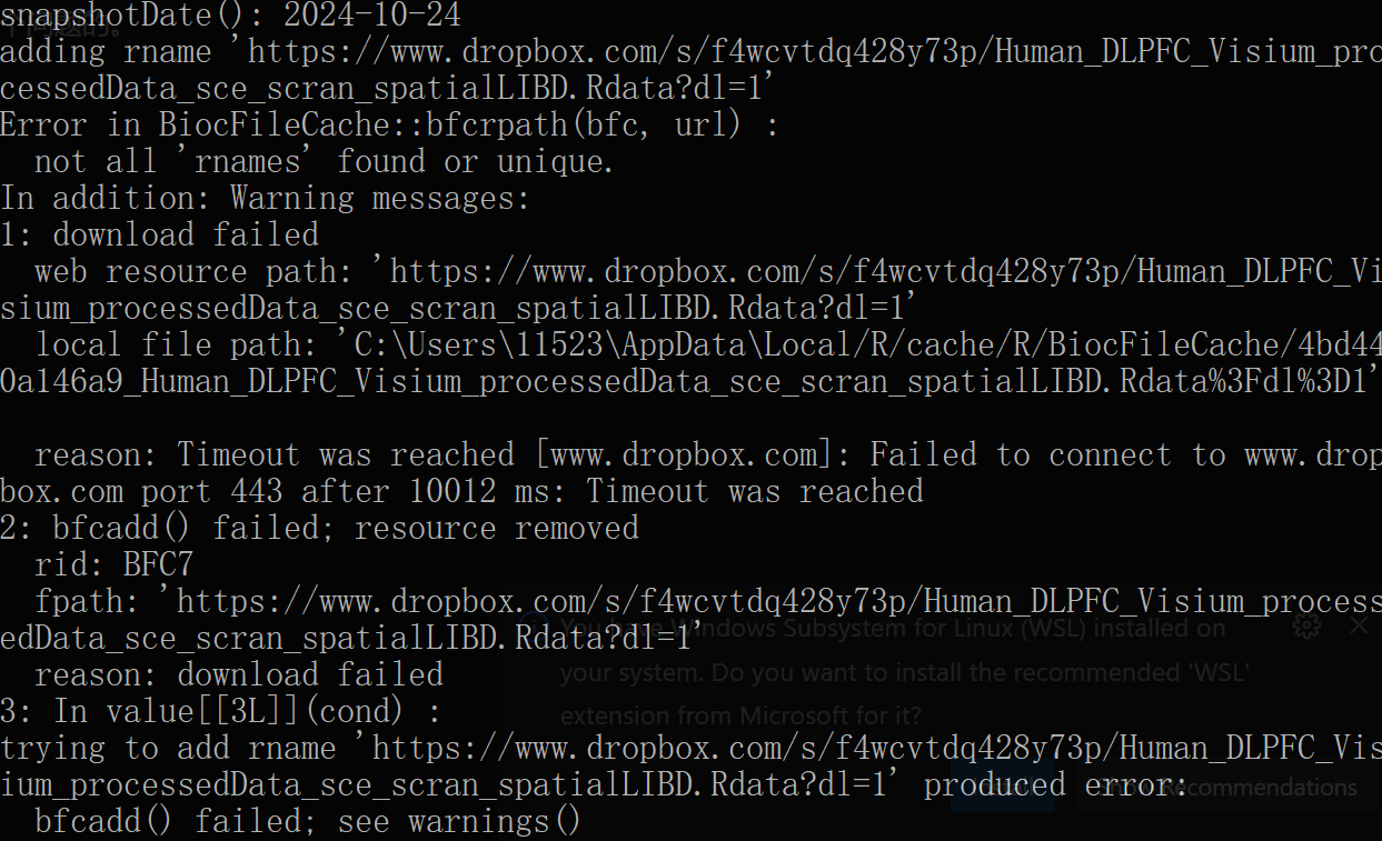
显然这个博主的链接时挂掉了，我重新尝试下载这个链接的内容发现没有办法下载，然而这个更新内容居然是直接把 spe 的数据链接更改成了 sce 的数据链接，也就是说从 Spatial 的数据变成了 Single Cell 的数据，然后最恶心的是这个 Single Cell 的数据是提供下载的，但是没有提供如何将这个数据转换成 Spatial 数据的方式，我摸索了半天，由于不会 R 语言只得放弃转换 Single Cell 数据这条路。

然后我便查阅这个所谓的 fetch_data 是怎么运行的，于是在运行

1	?fetch_data

后我来到了这个网页看到了这一段话

The initial version of spatialLIBD downloaded data only from https://github.com/LieberInstitute/HumanPilot.

结果，踏破铁鞋无觅处，得来全不费工夫，它实际上是直接提供了 spatial 数据的：

网址

事实上对于 spatial 文件夹的数据中的 csv 文件，也可以通过 python 去转换 txt 中的数据得到

import pandas as pd

# 文件路径
txt_file = "tissue_positions_list.txt"
csv_file = "tissue_positions_list.csv"

# 读取 txt 文件，假设以逗号分隔
df = pd.read_csv(txt_file, header=None)  # 默认没有表头

# 保存为 CSV 文件
df.to_csv(csv_file, index=False)

对于 h5ad 的数据可以在 spatialLIBD 网站中直接下载获取，对于 groud_truth 数据也可以提供的网站中下载，这里就不赘述了

在运行 pyG 的代码时出现了莫名其妙的错误，它提示我的图（意思是节点的引用超出了它本身的限制）有问题，

1	InternalError: Error at src/constructors/basic_constructors.c:75: Invalid (negative or too large) vertex ID. -- Invalid vertex ID

于是我转回到 tensorflow 的那个版本去运行，结果发现版本太高了

下面是解决方案：
网站

结果无论是 pyG 的代码还是 tensorflow 的代码，始终没有办法解决图的问题，我使用了我找的数据和网上给出的数据都没有办法解决这个问题，后面再看看是怎么回事吧。

而且很奇怪的是 pyG 给出来的结果远远优于 tensorFlow 的结果，即便代码有差异也不应该差别这么大，例如 pyG 的 ARI=0.61 而 tensorflow 的仅有 0.44

这个文章现在复现了 1/10，各种问题层出不穷，光是找 DLFPC 的数据就花了好几天，这论文感觉有点管杀不管埋，有点逆天。

先在 tensorflow 上跑的代码，感觉效果不好，等 pyG 整理好了去 pyG 跑一次

整理 pyG 时最开始用的是支持 GPU 的版本，结果调了半天 torch-sparse 总是不对，后来换成 CPU 的版本就行了，可能是我自己电脑的问题吧

整理完 pyG 发现跑不了这个模块的代码，理由是虽然本质上 pyG 和 tensorflow 版本是同一方法的不同实现，但是它的接口的变量没有同一，例如在 tensorflow 又 attention 的变量，但在 pyG 中没有设置，这真是管杀不管埋了，其实想要这个变量也很简单，重新写一下它 pyG 的代码就行了，但我现在只想快点结束这坨屎山代码，就不弄了，原理什么的已经很清楚了。

后面的几个 tutorial 有点不想弄了，本质上就是那几个函数在那捣鼓，具体看看 3D sptial domain 和 denoising 就暂时不弄了，反正毕业设计还得回来看。

不做了，弄下一篇去了，感觉继续复现下去也没有意义。

生物学习笔记类算法